ROI Analysis

ROI Analysis

VoltRon is capable of analyzing readouts from distinct spatial technologies including segmentation (ROI)-based transciptomics assays that capture large polygonic regions on tissue sections. VoltRon recognizes such readouts including ones from commercially available tools and allows users to implement a workflow similar to ones conducted on bulk RNA-Seq datasets. In this tutorial, we will analyze morphological images and gene expression profiles provided by the readouts of the Nanostring’s GeoMx Digital Spatial Profiler platform, a high-plex spatial profiling technology which produces segmentation-based protein and RNA assays.

In this use case, eight tissue micro array (TMA) tissue sections were fitted into the scan area of the slide loaded on the GeoMx DSP instrument. These sections were cut from control and COVID-19 lung tissues of donors categorized based on disease durations (acute and prolonged). See GSE190732 for more information.

You can download these tutorial files from here:

File	Link
Counts	DDC files
GeoMx Human Whole Transcriptome Atlas	Human RNA WTA for NGS
Segment Summary	ROI Metadata file
Morphology Image	Image file
OME.TIFF Image	OME.TIFF file
OME.TIFF Image (XML)	OME.TIFF (XML) file

We now import the GeoMx data, and start analyzing 87 user selected segments (i.e. region of interests, ROI) to check spatial localization of signals. The importGeoMx function requires:

• The path to the Digital Count Conversion file, dcc.path, and Probe Kit Configuration file, pkc.file, which are both provided as the output of the GeoMx NGS Pipeline.
• The path the to the metadata file, summarySegment, and the specific excel sheet that the metadata is found, summarySegmentSheetName, the path to the main morphology image and the original ome.tiff (xml) file, all of which are provided and imported from the DSP Control Center. Please see GeoMx DSP Data Analysis User Manual for more information.

library(VoltRon)
library(xlsx)
GeoMxR1 <- importGeoMx(dcc.path = "DCC-20230427/", 
                       pkc.file = "Hs_R_NGS_WTA_v1.0.pkc",
                       summarySegment = "segmentSummary.csv",
                       image = "Lu1A1B5umtrueexp.tif",
                       ome.tiff = "Lu1A1B5umtrueexp.ome.tiff.xml",
                       sample_name = "GeoMxR1")

We can import the GeoMx ROI segments from the Lu1A1B5umtrueexp.ome.tiff image file directly by replacing the .xml file with the .ome.tiff file in the ome.tiff argument. Note that you need to call the RBioFormats library. If you are getting a java error when running importGeoMx, try increasing the maximum heap size by supplying the -Xmx parameter. Run the code below before rerunning importGeoMx again.

options(java.parameters = "-Xmx4g")
library(RBioFormats)

Quality Control

Once the GeoMx data is imported, we can start off with examining key quality control measures and statistics on each segment to investigate each individual ROI such as sequencing saturation and the number of cells (nuclei) within each segment. VoltRon also provides the total number of unique transcripts per ROI and stores in the metadata.

library(ggplot2)
vrBarPlot(GeoMxR1, 
          features = c("Count", "Nuclei.count", "Sequencing.saturation"),
          x.label = "ROI.name", group.by = "ROI.type") + 
  theme(axis.text.x = element_text(size = 3))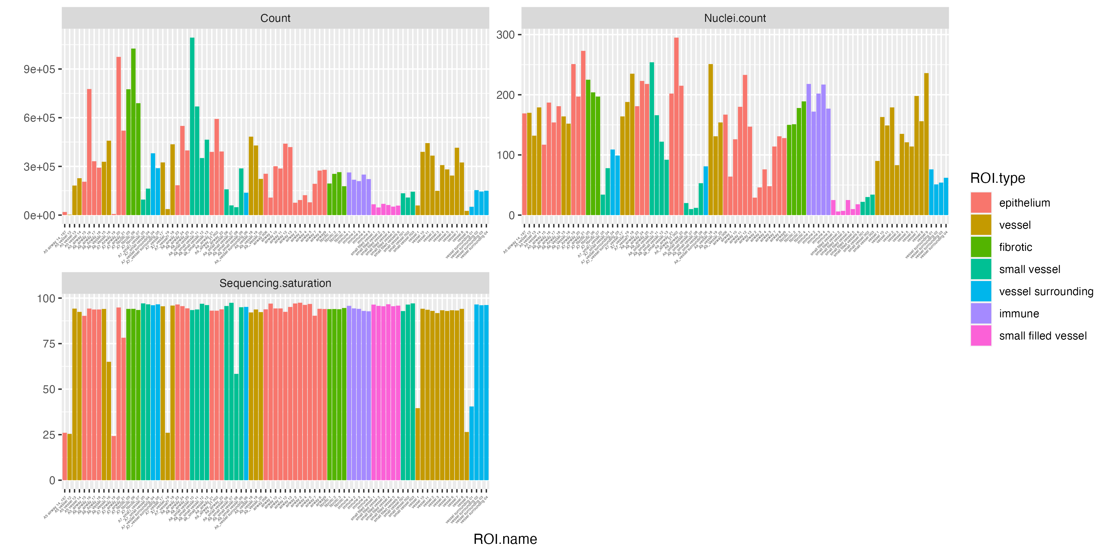

For measuring the quality of individual ROIs, we can add a new metadata column, called CountPerNuclei, to check the average quality of cells per ROI. It seems some number of ROIs with low counts per nuclei also have low sequencing saturation.

GeoMxR1$CountPerNuclei <- GeoMxR1$Count/GeoMxR1$Nuclei.count
vrBarPlot(GeoMxR1, 
          features = c("Count", "Nuclei.count", 
                       "Sequencing.saturation", "CountPerNuclei"),
          x.label = "ROI.name", group.by = "ROI.type", ncol = 2) + 
  theme(axis.text.x = element_text(size = 5))

Processing

We can now filter ROIs based on our earlier observation of them having low count per nuclei where some also have low sequencing saturation.

# Filter for count per nuclei
GeoMxR1 <- subset(GeoMxR1, subset = CountPerNuclei > 500)

We then filter genes with low counts by extracting the count matrix and putting aside all genes whose maximum count across all 87 ROIs are less than 10.

GeoMxR1_data <- vrData(GeoMxR1, norm = FALSE)
feature_ind <- apply(GeoMxR1_data, 1, function(x) max(x) > 10)
selected_features <- vrFeatures(GeoMxR1)[feature_ind]
GeoMxR1_lessfeatures <- subset(GeoMxR1, features = selected_features)

VoltRon is capable of normalizing data provided by a diverse set of spatial technologies, including the quantile normalization method suggested by the GeoMx DSP Data Analysis User Manual which scales the ROI profiles to the third quartile followed by the geometric mean of all third quartiles multipled to the scaled profile.

GeoMxR1 <- normalizeData(GeoMxR1, method = "Q3Norm")

Interactive Subsetting

Spatially informed genomic technologies heavily depend on image manipulation as images provide an additional set of information. Hence, VoltRon incorporates several interactive built-in utilities. One such functionality allows manipulating images of VoltRon assays where users can interactively choose subsets of images. However, we first resize the morphology image by providing the width of the new image (thus height will be reduced to preserve the aspect ratio).

# resizing the image
# GeoMxR1 <- resizeImage(GeoMxR1, size = 4000)

VoltRon provides a mini Shiny app for subsetting spatial points of a VoltRon object by using the image as a reference. This app is particularly useful when multiple tissue sections were fitted to a scan area of a slide, such as the one from GeoMx DSP instrument. We use interactive = TRUE option in the subset function to call the mini Shiny app, and select bounding boxes of each newly created subset. Please continue until all eight sections are selected and subsetted.

GeoMxR1_subset <- subset(GeoMxR1, interactive = TRUE)

We can now merge the list of subsets, or samples, each associated with one of eight sections. You can provide a list of names for the newly subsetted samples.

GeoMxR1_subset_list <- GeoMxR1_subset$subsets
GeoMxR1 <- merge(GeoMxR1_subset_list[[1]], GeoMxR1_subset_list[-1])
GeoMxR1

VoltRon Object 
prolonged case 4: 
  Layers: Section1 
acute case 3: 
  Layers: Section1 
control case 2: 
  Layers: Section1 
acute case 1: 
  Layers: Section1 
acute case 2: 
  Layers: Section1 
... 
There are 8 samples in total 
Assays: GeoMx(Main) GeoMx_NegProbe 

You may also save the selected image subsets and reproduce the interactive subsetting operation for later use.

samples <- c("prolonged case 4", "acute case 3", "control case 2", 
             "acute case 1", "acute case 2", "prolonged case 5", 
             "prolonged case 3", "control case 1")
subset_info_list <- GeoMxR1_subset$subset_info_list[[1]]
GeoMxR1_subset_list <- list()
for(i in 1:length(subset_info_list)){
  GeoMxR1_subset_list[[i]]  <- subset(GeoMxR1, image = subset_info_list[i])
  GeoMxR1_subset_list[[i]] <- samples[i]
}
GeoMxR1 <- merge(GeoMxR1_subset_list[[1]], GeoMxR1_subset_list[-1])

Visualization

We will now select sections of interests from the VoltRon object, and visualize ROIs and features for each of these sections.

The function vrSpatialPlot plots categorical attributes associated with ROIs. In this case, we will visualize types of ROIs that were labelled and annotated during ROI selection.

GeoMxR1_subset <- subset(GeoMxR1, sample = c("prolonged case 4","acute case 3"))
vrSpatialPlot(GeoMxR1_subset, group.by = "ROI.type", ncol = 3, alpha = 0.6)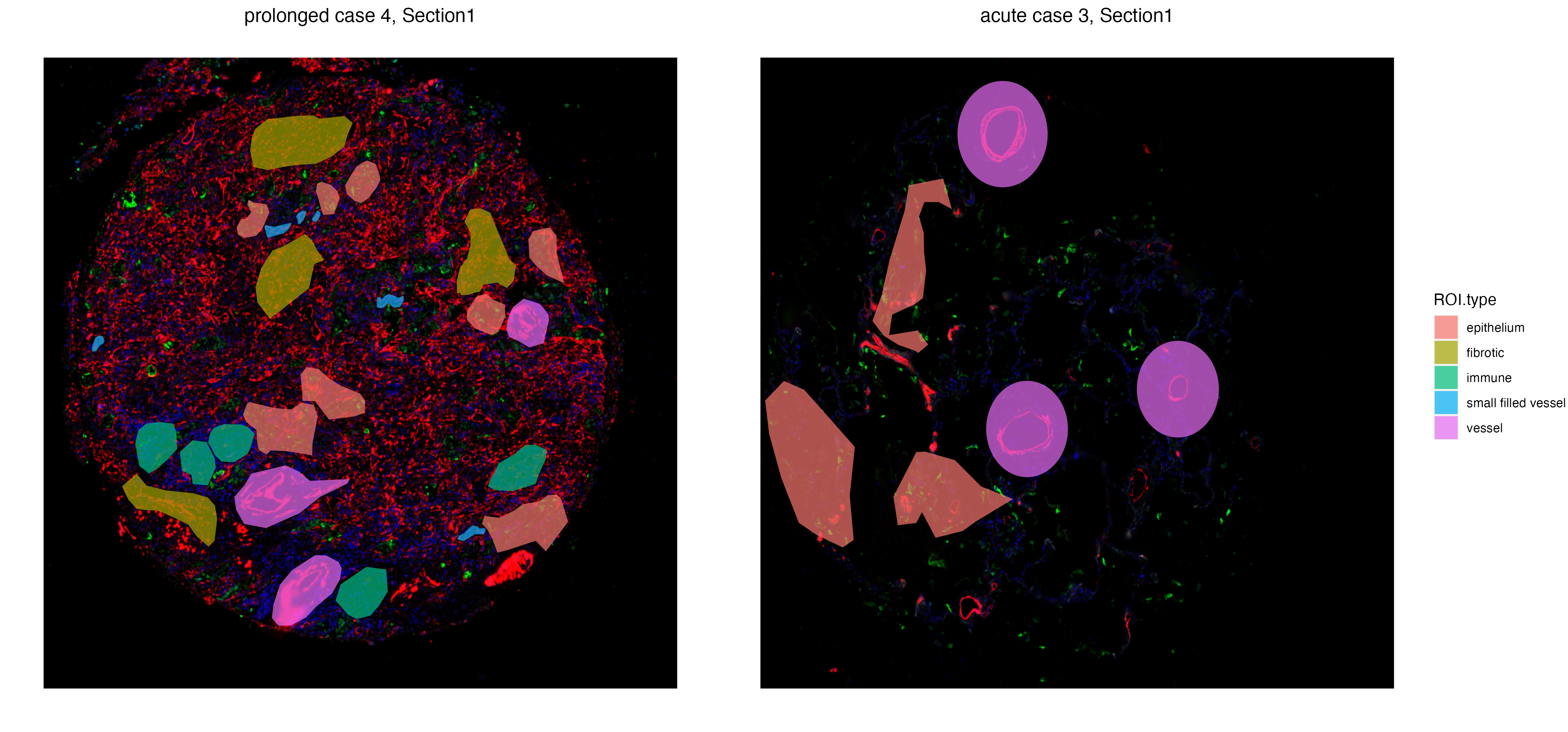

The function vrSpatialFeaturePlot detects the number of assays within each VoltRon object and visualizes each feature per each spatial image. A grid of images are visualized either the number of assays or the number of features are larger than 1. Here, we visualize the normalized expression of COL1A1 and C1S, two fibrotic markers, across ROIs of two prolonged covid cases. One may observe that the fibrotic regions of prolonged case 5 have considerably more COL1A1 and C1S compared to prolonged case 4.

GeoMxR1_subset <- subset(GeoMxR1, sample = c("prolonged case 4","prolonged case 5"))
vrSpatialFeaturePlot(GeoMxR1_subset, features = c("COL1A1", "C1S"), group.by = "ROI.name", 
                     log = TRUE, label = TRUE, keep.scale = "feature", title.size = 15)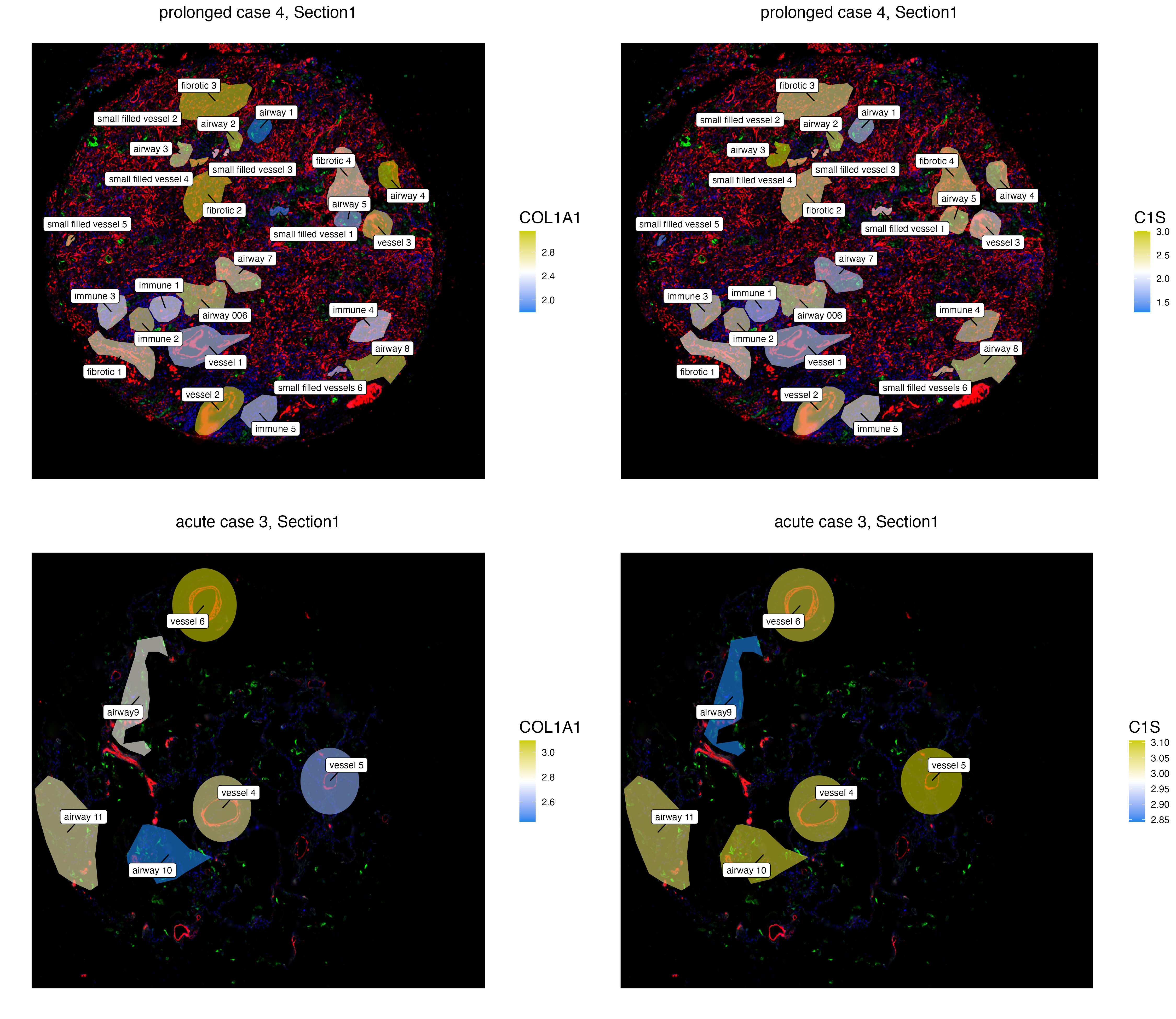

Dimensionality Reduction

We can now process the normalized and demultiplexed samples to map ROIs across all sections onto lower dimensional spaces. The functions getFeatures and getPCA select features (i.e. genes) of interest from the data matrix across all samples and reduce it to a selected number of principal components.

GeoMxR1 <- getFeatures(GeoMxR1)
GeoMxR1 <- getPCA(GeoMxR1, dims = 30)

The function vrEmbeddingPlot can be used to visualize embedding spaces (pca, umap, etc.) for any spatial point supported by VoltRon, hence cells, spots and ROI are all visualized using the same set of functions. Here we generate a new metadata column that represents the disease durations (control, acute and prolonged case), then map gene profiles to the first two principal components.

GeoMxR1$Condition <- gsub(" [0-9]+$", "", GeoMxR1$Sample)
vrEmbeddingPlot(GeoMxR1, group.by = c("Condition"), embedding = "pca", pt.size = 3)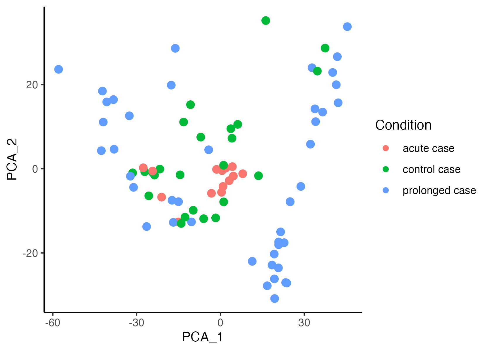

VoltRon provides additional dimensionality reduction techniques such as UMAP.

GeoMxR1 <- getUMAP(GeoMxR1)

Gene expression profiles of ROIs associated with prolonged case sections seem to show some heterogeneity. We now color segments by section (or replicate, Sample) to observe the sources of variability. Three replicates of prolonged cases exhibit three different clusters of ROIs.

vrEmbeddingPlot(GeoMxR1, group.by = c("Condition"), embedding = "pca", pt.size = 3)
vrEmbeddingPlot(GeoMxR1, group.by = c("ROI.type"), embedding = "pca", pt.size = 3)
vrEmbeddingPlot(GeoMxR1, group.by = c("ROI.type"), embedding = "umap", pt.size = 3)

Differential Expression Analysis

VoltRon provides wrapping functions for calling tools and methods from popular differential expression analysis package such as DESeq2. We utilize DESeq2 to find differentially expressed genes across each pair of ROI types conditions.

# get DE for all conditions
library(DESeq2)
library(dplyr)
DEresults <- getDiffExp(GeoMxR1, group.by = "ROI.type",
                        group.base = "vessel", method = "DESeq2")
DEresults_sig <- DEresults %>% filter(!is.na(padj)) %>% 
  filter(padj < 0.05, abs(log2FoldChange) > 1)
head(DEresults_sig)

         baseMean log2FoldChange     lfcSE     stat       pvalue         padj     gene             comparison
ACTA2    33.48395       1.508701 0.3458464 4.362343 1.286768e-05 4.902586e-03    ACTA2 ROI.type_vessel_epithelium
ADAMTS1  22.29160       1.152556 0.2272085 5.072680 3.922515e-07 4.109815e-04  ADAMTS1 ROI.type_vessel_epithelium
C11orf96 27.48924       1.142085 0.3041057 3.755554 1.729585e-04 2.588819e-02 C11orf96 ROI.type_vessel_epithelium
CNN1     16.87670       1.112662 0.2680222 4.151381 3.304757e-05 9.766004e-03     CNN1 ROI.type_vessel_epithelium
CRYAB    21.85960       1.264747 0.2173272 5.819552 5.900570e-09 2.472929e-05    CRYAB ROI.type_vessel_epithelium
FLNA     44.50957       1.270025 0.3243115 3.916066 9.000548e-05 1.985331e-02     FLNA ROI.type_vessel_epithelium

The vrHeatmapPlot takes a set of features for any type of spatial point (cells, spots and ROIs) and visualizes scaled data per each feature. We select highlight.some = TRUE to annotate features which could be large in size where you can also select the number of such highlighted genes with n_highlight. There seems to be two groups of fibrotic regions that most likely associated with two prolonged case samples.

# get DE for all conditions
library(ComplexHeatmap)
vrHeatmapPlot(GeoMxR1, features = unique(DEresults_sig$gene), group.by = "ROI.type", 
              highlight.some = TRUE, n_highlight = 40)

In order to get a deeper understanding of differences between fibrotic regions across two prolonged case replicates. We first subset the GeoMx data to only sections with fibrotic ROIs.

fibrotic_ROI <- vrSpatialPoints(GeoMxR1)[GeoMxR1$ROI.type == "fibrotic"]
GeoMxR1_subset <- subset(GeoMxR1, spatialpoints = fibrotic_ROI)
vrSpatialPlot(GeoMxR1_subset, group.by = "ROI.type", ncol = 3, alpha = 0.4)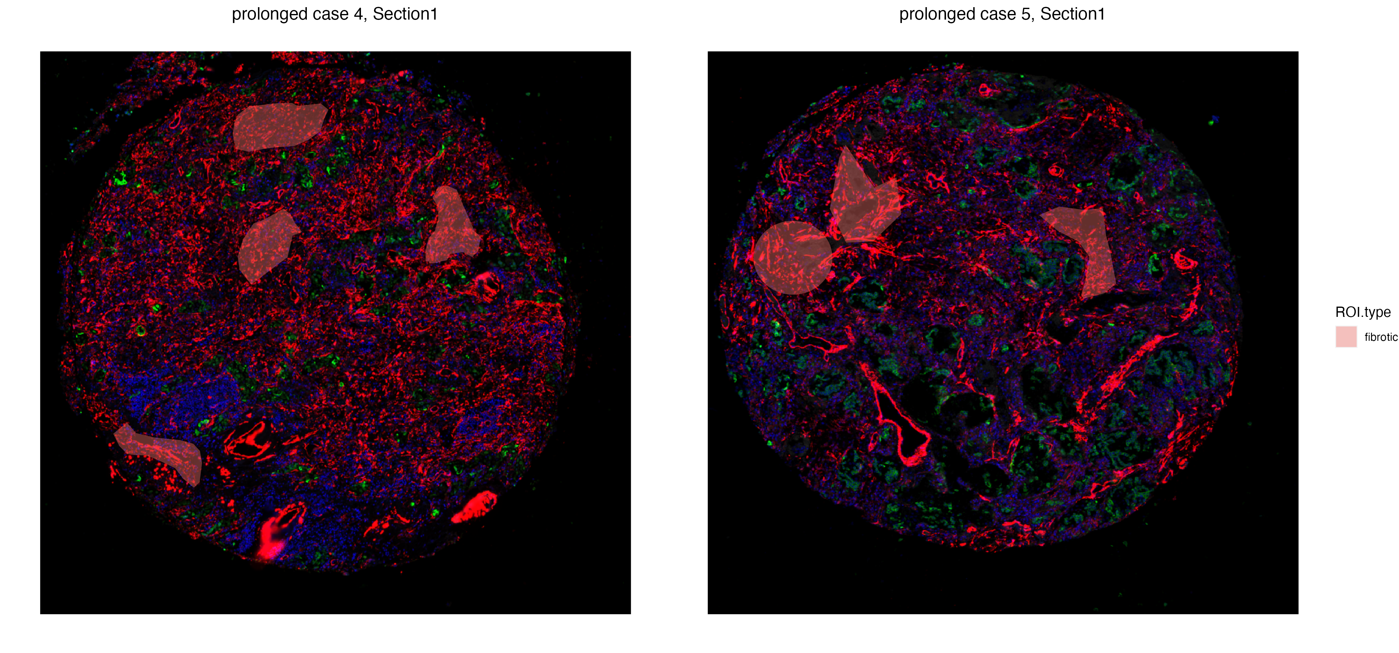

The getDiffExp function is capable of testing differential expression across all metadata columns, including the Samples column that captures labels of different tissue sections. Macrophage markers such as CD68 and CD163 are differentially expressed in fibrotic regions of case 5 compared to case 4, including FN1, a profibrotic gene whose expression can be found on macrophages.

DEresults <- getDiffExp(GeoMxR1_subset, group.by = "Sample", 
                        group.base = "prolonged case 5", method = "DESeq2")
DEresults_sig <- DEresults %>% filter(!is.na(padj)) %>%
  filter(padj < 0.05, abs(log2FoldChange) > 1)
DEresults_sig <- DEresults_sig[order(DEresults_sig$log2FoldChange, decreasing = TRUE),]
head(DEresults_sig)

       baseMean log2FoldChange     lfcSE      stat       pvalue         padj   gene                               comparison
COL3A1 708.5599       6.635411 0.5198805 12.763338 2.626978e-37 1.596809e-33 COL3A1 Sample_prolonged case 5_prolonged case 4
COL1A2 836.0790       5.237228 0.4407380 11.882861 1.453071e-32 4.416246e-29 COL1A2 Sample_prolonged case 5_prolonged case 4
COL1A1 460.2184       5.175153 0.5237868  9.880267 5.069785e-23 3.081669e-20 COL1A1 Sample_prolonged case 5_prolonged case 4
FN1    278.6594       5.083687 0.3717299 13.675754 1.417301e-42 1.723013e-38    FN1 Sample_prolonged case 5_prolonged case 4
HBB    202.7693       4.944228 0.4884175 10.122955 4.370193e-24 3.794888e-21    HBB Sample_prolonged case 5_prolonged case 4
A2M    466.4328       4.925236 0.4542682 10.842133 2.173435e-27 3.774636e-24    A2M Sample_prolonged case 5_prolonged case 4

ROI Deconvolution

VoltRon supports multiple bulk RNA deconvolution algorithms to analyze the cellular composition of both ROIs and spots. In order to integrate the scRNA data and the GeoMx data sets within the VoltRon objects, we will use the MuSiC package. We will use a human lung scRNA dataset (GSE198864) as reference, which is found here.

set.seed(1)
library(Seurat)
library(SingleCellExperiment)
seu <- readRDS("GSE198864_lung.rds")
scRNAlung <- seu[,sample(1:ncol(seu), 10000, replace = FALSE)]

DimPlot(scRNAlung, reduction = "umap", label = T, group.by = "Clusters") + NoLegend()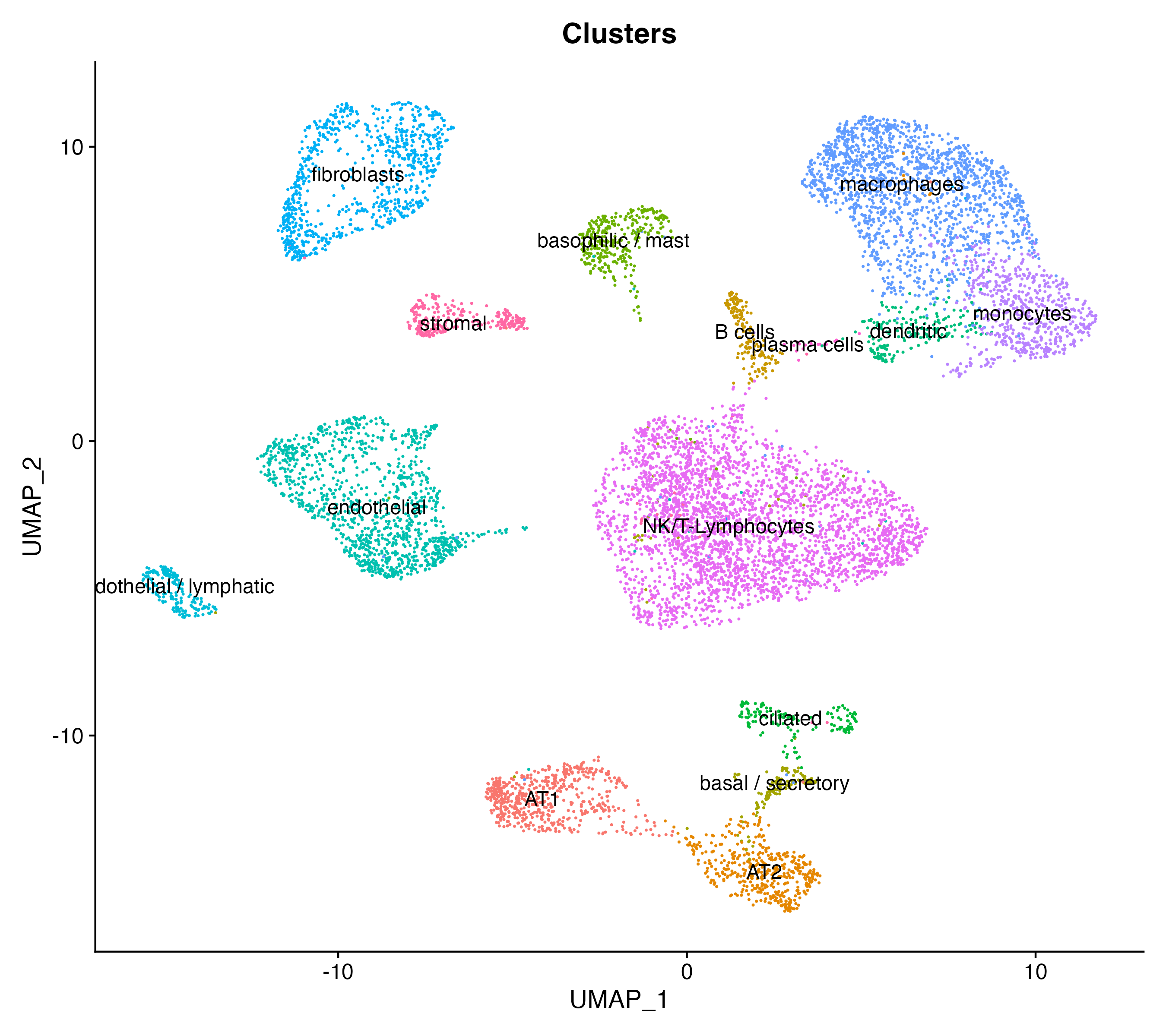

We utilize the getDeconvolution function to call wrapper functions for deconvolution algorithms (see ). For all layers with GoeMx assays, an additional assay within the same layer with _decon postfix will be created. The sc.object argument can either be a Seurat or SingleCellExperiment object.

library(MuSiC)
GeoMxR1 <- getDeconvolution(GeoMxR1,
                            sc.object = scRNAlung, sc.assay = "RNA", 
                            sc.cluster = "Clusters", sc.samples = "orig.ident")
SampleMetadata(GeoMxR1)

              Assay    Layer           Sample
Assay1        GeoMx Section1 prolonged case 4
Assay2        GeoMx Section1     acute case 3
Assay3        GeoMx Section1   control case 2
Assay4        GeoMx Section1     acute case 1
Assay5        GeoMx Section1     acute case 2
Assay6        GeoMx Section1 prolonged case 5
Assay7        GeoMx Section1 prolonged case 3
Assay8        GeoMx Section1   control case 1
Assay9  GeoMx_decon Section1 prolonged case 4
Assay10 GeoMx_decon Section1     acute case 3
Assay11 GeoMx_decon Section1   control case 2
Assay12 GeoMx_decon Section1     acute case 1
Assay13 GeoMx_decon Section1     acute case 2
Assay14 GeoMx_decon Section1 prolonged case 5
Assay15 GeoMx_decon Section1 prolonged case 3
Assay16 GeoMx_decon Section1   control case 1

We can now visualize cell type compositions of each ROI. Before running vrProportionPlot function, we need to set the main assay as GeoMx_decon. One may see the increased proportion of cells NK cells and T cells in immune ROIs.

vrMainAssay(GeoMxR1) <- "GeoMx_decon"
vrProportionPlot(GeoMxR1)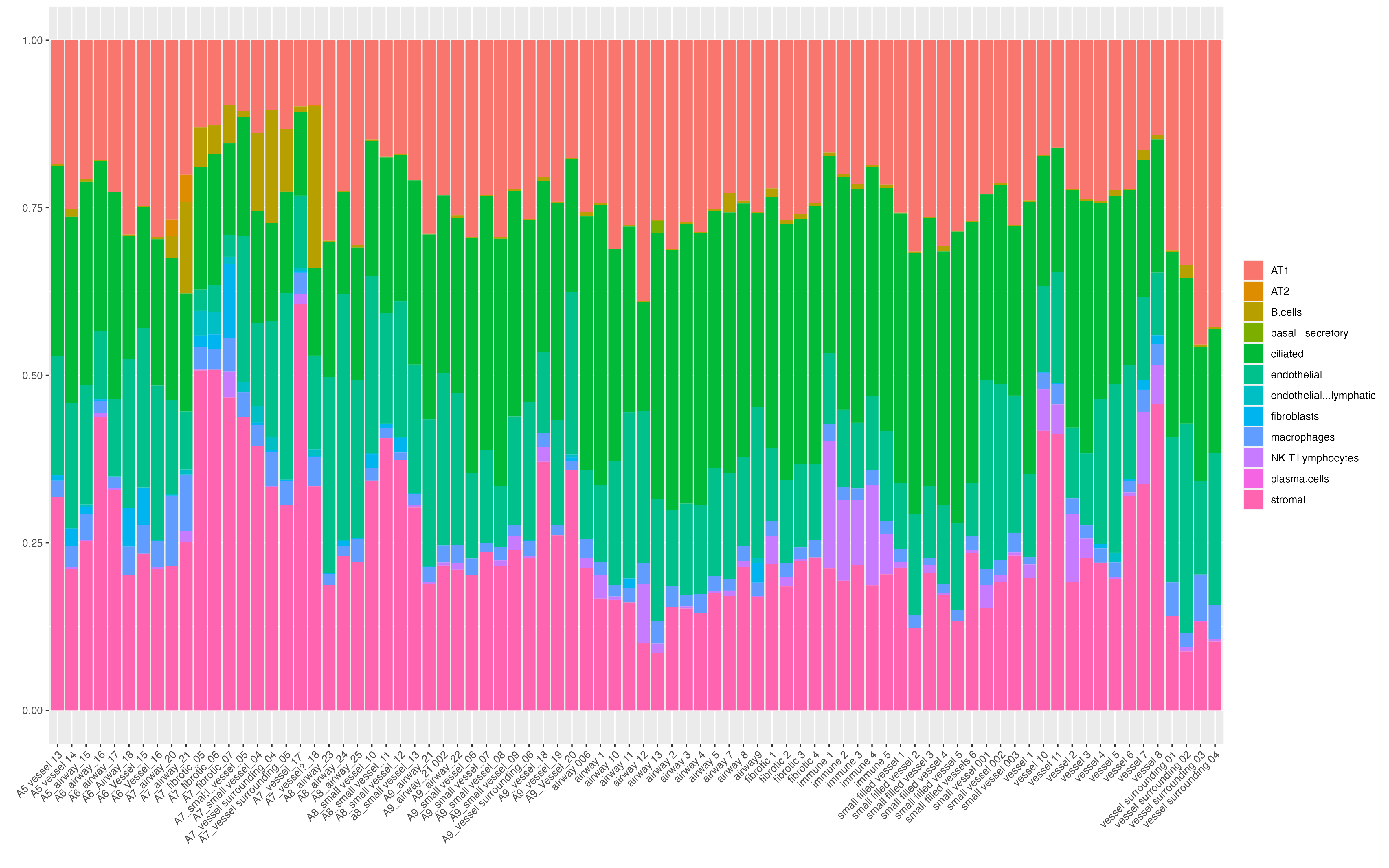

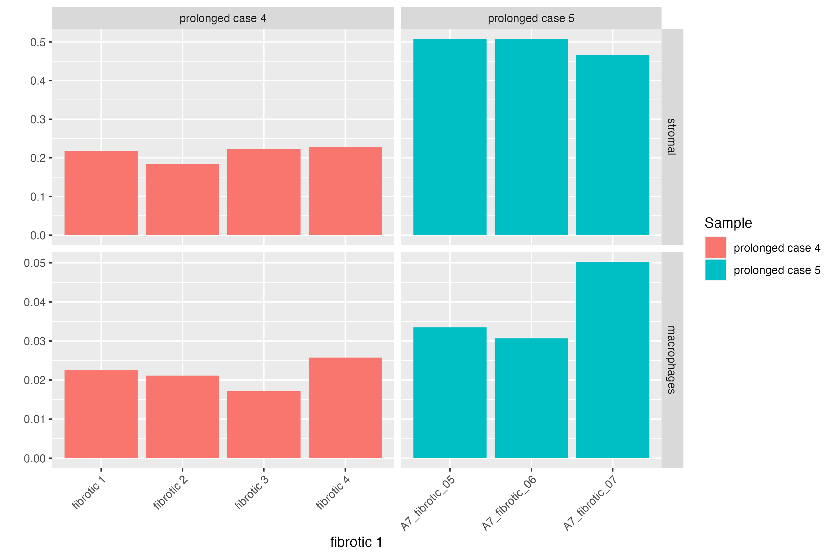
Here, we can subset the GeoMx object further to dive deep into the cellular proportions of each fibrotic region of prolonged cases. Comparing prolonged case 5 against case 4, we see an increase in the cellular population of the stromal cluster defined in Mothes et. al 2023 (that are both vascular and airway smooth muscle cells), and an increase abundance of macrophages which may indicate that these macrophages are profibrotic being within and close to fibrotic regions with increased gene expression of FN1.

# subsetting fibrotic regions
spatialpoints <- vrSpatialPoints(GeoMxR1)[GeoMxR1$ROI.type == "fibrotic"]
GeoMxR1_subset <- subset(GeoMxR1, spatialpoints = spatialpoints)

# Proportion plot
vrProportionPlot(GeoMxR1_subset, x.label = "ROI.name", split.method = "facet_grid", 
                 split.by = "Sample")

# barplot 
vrBarPlot(GeoMxR1_subset, features = c("stromal", "macrophages"), group.by = "Sample",
          x.label = "ROI.name", split.by = "Sample")

H&E Image Integration

Questions may arise when these ROI that are initially annotated as fibrotic regions may in fact be fibrotic. VoltRon provides advanced image registration workflows which we can use to H&E images of from the same TMA blocks where GeoMx slides were established.

We first import the H&E image of the prolonged case 4 TMA section using the importImageData function. This will import the H&E image as a standalone VoltRon object. For more information on image-based VoltRon objects, see the Downstream analysis of Pixels section.

We will use the H&E image of TMA section taken from the same block as the Prolonged case 4. You can download the image from here.

vrHEimage <- importImageData("prolonged_case4_HE.tif", image_name = "H&E")
vrImages(vrHEimage, scale.perc = 40)

We can now register the GeoMx slide with the newly imported H&E based VoltRon object. Since two images are associated with TMA sections that are not adjacent, we have to rely on the localization of vessels visible in both images for alignment. VoltRon allows manipulating multiple channels of an image object two choose the best background image for manual landmark selection. For more information on both manual and automated registration of VoltRon objects, see here.

GeoMxR1_subset <- subset(GeoMxR1, sample = c("prolonged case 4"))
GeoMxReg <- registerSpatialData(reference_spatdata = GeoMxR1_subset, query_spatdata = vrHEimage)

The result of the registration is a list of registered VoltRon objects which we can use for parsing the registered image as well. In this case, the second element of the resulting list would be the registered H&E based VoltRon object. We can also exchange images where the H&E image now is registered to the perspective as the GeoMx channels, and can be defined as a new channel in the original GeoMx object.

vrHEimage_reg <- GeoMxReg$registered_spat[[2]]
vrImages(GeoMxR1_subset[["Assay1"]], name = "image_1", channel = "H&E") <- vrImages(vrHEimage_reg, name = "H&E_reg")

We can now visualize the ROIs and their annotations where the registered H&E visible in the background. We define the image key image_1 and the channel name H&E.

vrSpatialPlot(GeoMxR1_subset, group.by = "ROI.type", alpha = 0.7, background = c("image_1", "H&E"))

Interactive Visualization can also be used to zoom in to ROIs and investigate the pathology associated with GeoMx ROIs labeled as fibrotic.

vrSpatialPlot(GeoMxR1_subset, group.by = "ROI.type", alpha = 0.7, background = c("image_1", "H&E"), interactive = TRUE)