Interactive
Interactive Annotation
VoltRon includes interactive applications to select and manually label spatial points by drawing polygons and circles. As an example, we will use a Spot-based spatial transcriptomics assay, specifically the Mouse Brain Serial Section 1/2 datasets, analyzed in the Niche Clustering tutorial. You can find the already analyzed data stored as a VoltRon object here
MBrain_Sec <- readRDS("Visium&Visium_data_decon_analyzed.rds")We can start annotating the spatial assay. By passing arguments used by the vrSpatialPlot function to visualize labels (e.g. clusters), we can better select regions within tissue sections for annotation.
MBrain_Sec <- annotateSpatialData(MBrain_Sec, assay = "Assay1",
                                  group.by = "clusters", label = "annotation")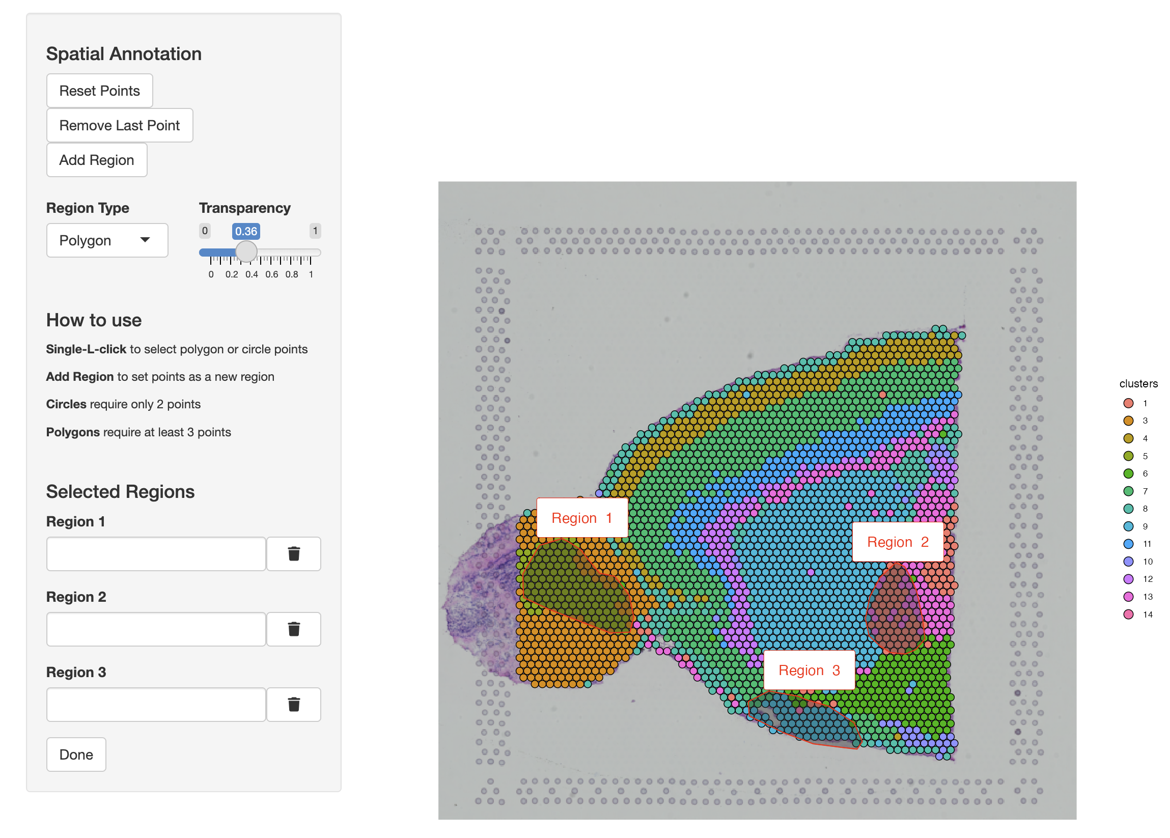
Here, annotateSpatialData function not only labels spots with within regions of interests (ROIs) selected by the user, but also records these regions in ROI assays within the same layer of the annotated Visium assay. The new assay type will be given the name ROIAnnotations if otherwise not specified using the annotation_assay argument in the function.
MBrain_Sec VoltRon Object
Anterior:
Layers: Section1 Section2
Posterior:
Layers: Section1 Section2
Assays: Visium_decon(Main) Visium ROIAnnotation MBrain_Sec@sample.metadata > MBrain_Sec@sample.metadata
Assay Layer Sample
Assay1 Visium Section1 Anterior
Assay2 Visium Section2 Anterior
Assay3 Visium Section1 Posterior
Assay4 Visium Section2 Posterior
Assay5 ROIAnnotation Section1 AnteriorThe new annotations are available in the metadata of the spot assay (default assay in this object) and can be visualized if wanted.
head(Metadata(MBrain_Sec)) Count Assay Layer Sample clusters annotation
AAACAAGTATCTCCCA-1_Assay1 1 Visium_decon Section1 Anterior 1 Region 3
AAACACCAATAACTGC-1_Assay1 1 Visium_decon Section1 Anterior 3 undefined
AAACAGAGCGACTCCT-1_Assay1 1 Visium_decon Section1 Anterior 4 undefined
AAACAGCTTTCAGAAG-1_Assay1 1 Visium_decon Section1 Anterior 5 Region 1
AAACAGGGTCTATATT-1_Assay1 1 Visium_decon Section1 Anterior 5 Region 1
AAACATGGTGAGAGGA-1_Assay1 1 Visium_decon Section1 Anterior 3 undefinedvrSpatialPlot(MBrain_Sec, assay = "Assay1", group.by = "annotation")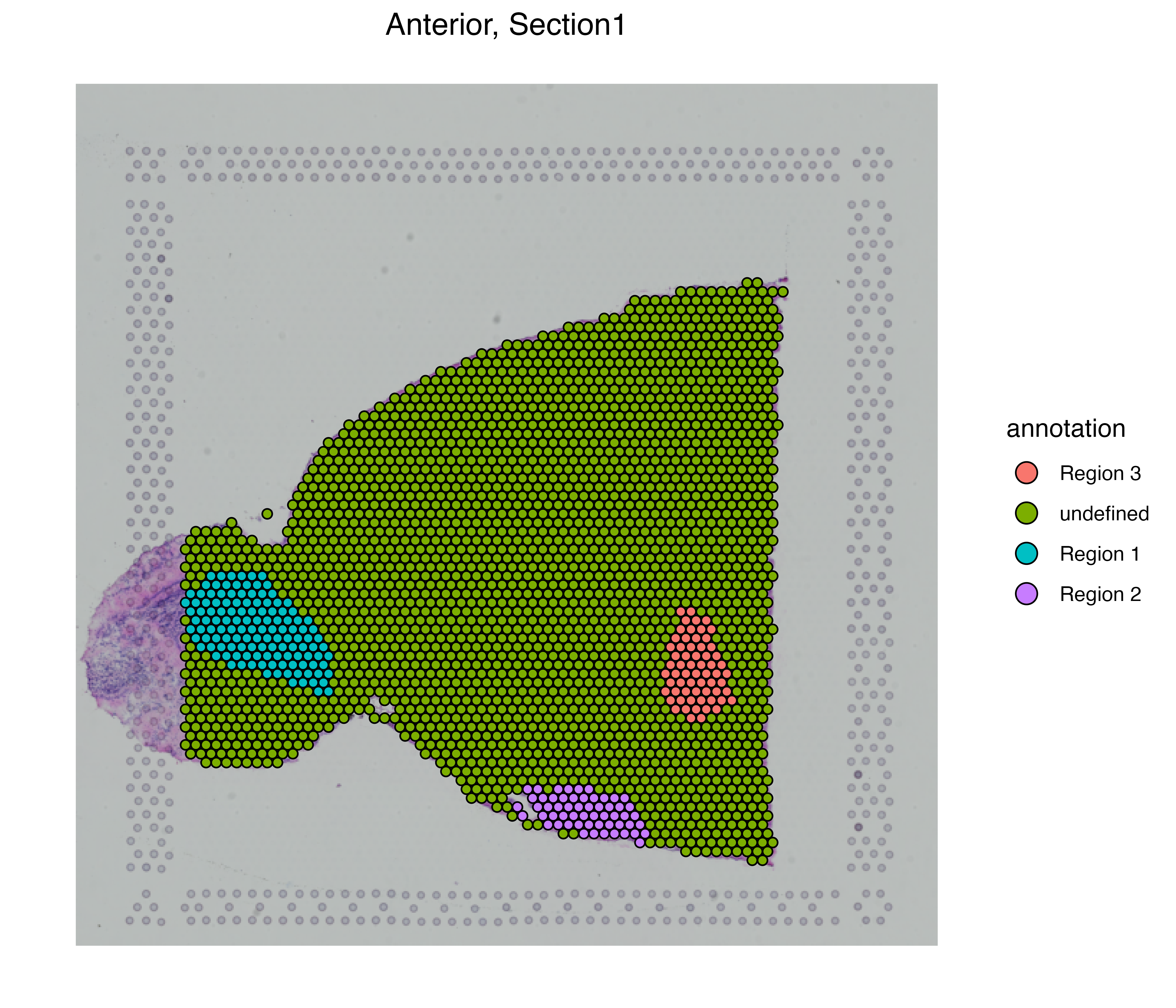
You can also overlay the ROI annotations with the clustered spots to visualize multiple assays at the same time.
library(ggnewscale)
vrSpatialPlot(MBrain_Sec, assay = "Assay1", group.by = "clusters") |>
  addSpatialLayer(MBrain_Sec, assay = "Assay5", group.by = "annotation", alpha = 0.7)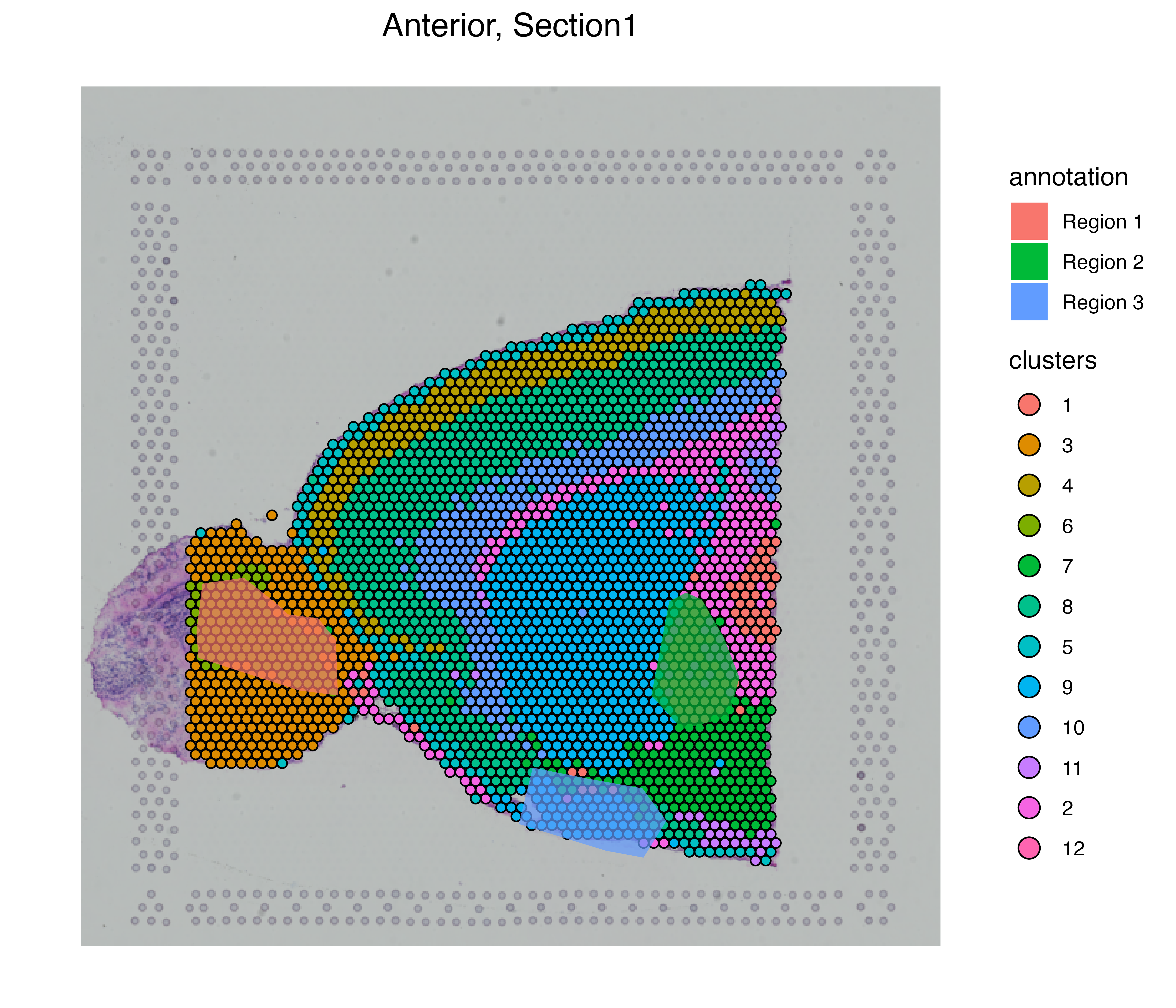
Interactive Visualization
VoltRon incorporates utilities
- (i) to convert VoltRon objects into other spatial data objects and files that could be used by platforms, and
- (ii) to incorporate wrapper functions to call methods from packages that support interactive visualization
Vitessce
We will transform VoltRon objects of Xenium data into zarr arrays, and use them for interactive visualization in Vitessce. We should first download the vitessceR package which incorporates wrapper function to visualize zarr arrays interactively in R.
if (!require("devtools", quietly = TRUE))
    install.packages("devtools")
if (!require("vitessceR", quietly = TRUE))
    devtools::install_github("Artur-man/vitessceR")
We can convert the VoltRon object into an AnnData object and save it as a a zarr array using the as.AnnData function which will create the array in the specified location. We use the flip_coordinates=TRUE argument to flip the coordinates of cells vertically, hence match it with the top to bottom system of the background DAPI image. Also, we can save an OMETIFF file of the DAPI image using create.ometiff argument to be used by vitessceR later.
data(xenium_data)
xenium_data <- as.AnnData(xenium_data, file = "xenium_data.zarr", assay = "Xenium",
                          flip_coordinates = TRUE, create.ometiff = TRUE)
We can use the zarr file directly in the vrSpatialPlot function to visualize the zarr array interactively in RStudio viewer. The reduction argument allows the umap of the Xenium data to be visualized alongside with the spatial coordinates of the Xenium cells (thus associated cell segmentations).
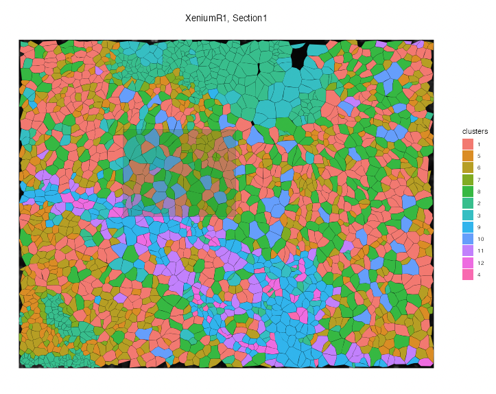
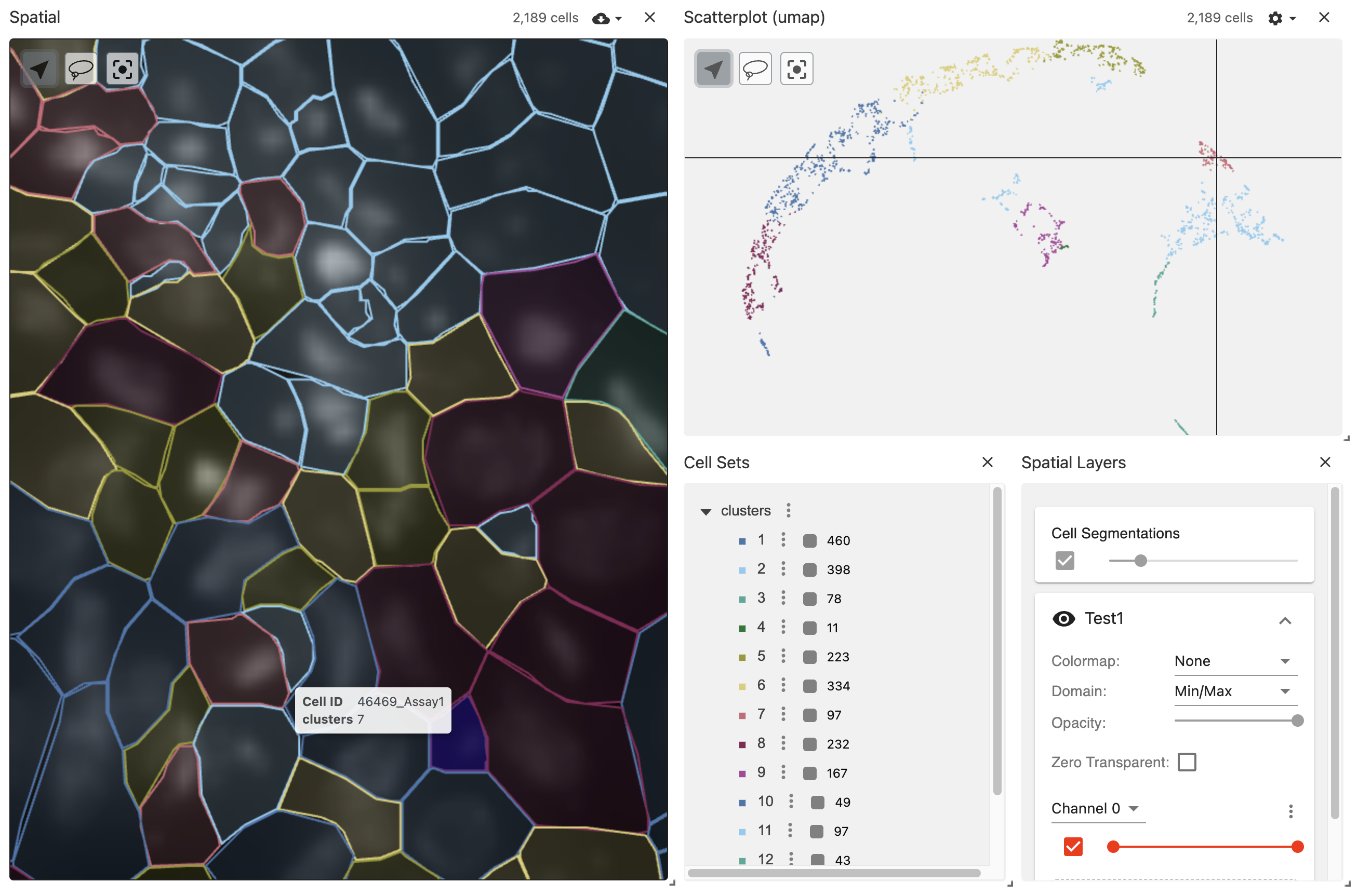
vrSpatialPlot("xenium_data.zarr", group.by = "clusters", reduction = "umap")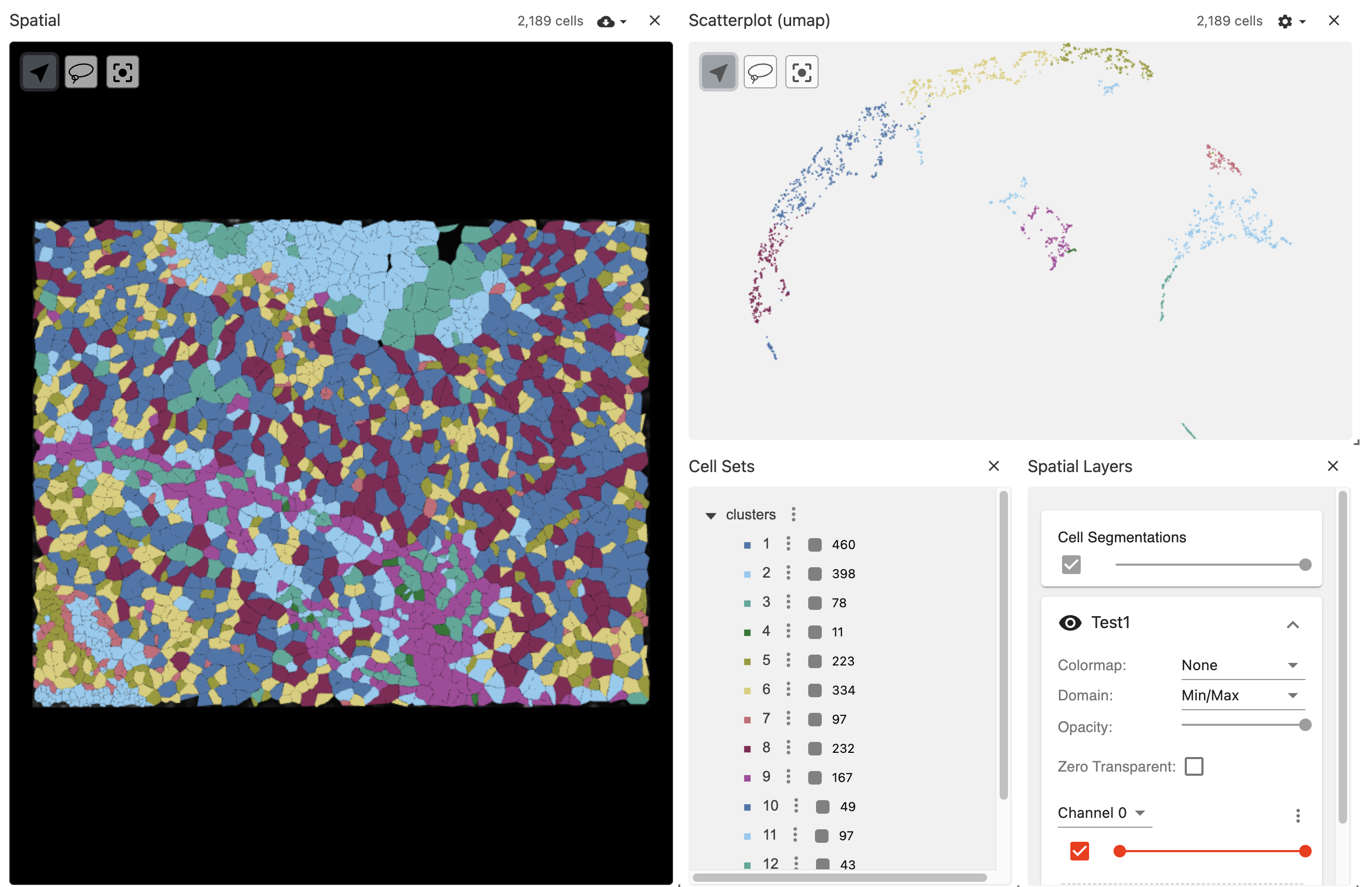
The vitessce application in the viewer pane allows visualizing background DAPI image and segmentations simultaneously while allowing users to zoom in and control the pane for advanced visualization.
TissUUmaps
To use TissUUmaps for interactive investigation of your spatial omics data, we first need to convert the VoltRon object into an AnnData object. However, this time we save the AnnData object as an h5ad array using again the as.AnnData function which will create the array in the specified location. We use the flip_coordinates=TRUE argument to flip the coordinates of cells vertically, hence match it with the top to bottom system of the background DAPI image.
data(xenium_data)
as.AnnData(xenium_data, file = "xenium_data.h5ad", assay = "Xenium", flip_coordinates = TRUE)
To use TissUUmaps, you can follow the instructions here. Once installed and executed, simply drag and drop the h5ad file to the main panel of the application
VoltRon
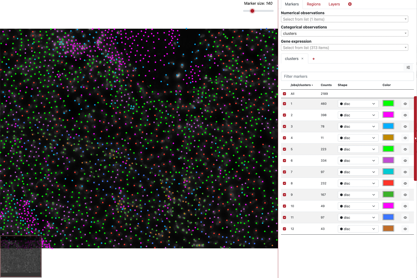
You can also use the built-in Shiny-based interactive visualizers of the VoltRon package by calling interactive=TRUE. You can zoom in by drawing a box on the plot and double-clicking in the selected area.
vrSpatialPlot(xenium_data, group.by = "clusters", plot.segments = TRUE, interactive = TRUE)