Image Registration
Spatial Data Alignment
Spatial genomics technologies often generate diverse images and spatial readouts, even though the tissue slices are from adjacent sections of a single tissue block. Hence, the alignment of images and spatial coordinates across tissue sections are of utmost importance to dissect the correct spatial closeness across these sections.
VoltRon allows users to align spatial omics datasets of these serial sections for data transfer and 3 dimensional stack alignment. The order of the tissue/sample slices should be provided by the user. VoltRon provides a fully embedded shiny application to either automatically or manually align images. The automatic alignment is achieved with the OpenCV’s C++ library fully embedded in the VoltRon package.
|
|
Alignment of Xenium and Visium
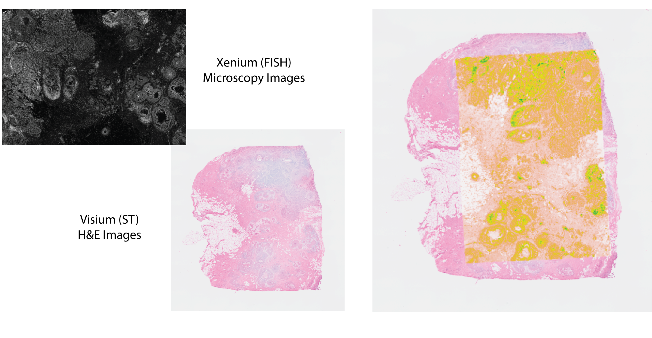
In this use case, we will align immunofluorescence (IF) and H&E images of the Xenium In Situ and Visium CytAssist platforms readouts. Three tissue sections are derived from a single formalin-fixed, paraffin-embedded (FFPE) breast cancer tissue block. A 5 \(\mu\)m section was taken for Visium CytAssist and two replicate 5 \(\mu\)m sections were taken for the Xenium replicates. More information on the spatial datasets and the study can be also be found on the BioRxiv preprint.
You can download the Xenium and Visium readouts from the 10x Genomics website (specifically, import In Situ Replicate 1/2 and Visium Spatial). Alternatively, you can download a zipped collection of three Visium and Xenium readouts from here.
VoltRon includes built-in functions for converting readouts from both Xenium and Visium platforms into VoltRon objects. We will import both Xenium replicates alongside with the Visium CytAssist data so that we can register images of these assays and merge them into one VoltRon object.
# dependencies
if(!requireNamespace("RBioFormats"))
  BiocManager::install("RBioFormats")
if(!requireNamespace("arrow"))
  install.packages("arrow")
if(!requireNamespace("rhdf5"))
  BiocManager::install("rhdf5")
library(VoltRon)

# import Xenium data
Xen_R1 <- importXenium("Xenium_R1/outs", sample_name = "XeniumR1")
Xen_R2 <- importXenium("Xenium_R2/outs", sample_name = "XeniumR2")

# import Visium data
Vis <- importVisium("Visium/", sample_name = "VisiumR1")
Before moving on to image alignment, we can inspect both Xenium and Visium images. We use the vrImages function to call and visualize reference images of all VoltRon objects.
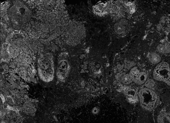
vrImages(Xen_R1)
vrImages(Xen_R2)
vrImages(Vis)
|
|
|
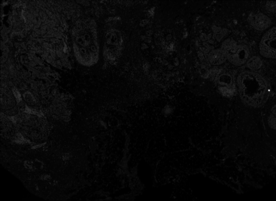
Although images of the first Xenium replicate and the Visium assay are workable, we have to adjust the brightness of the second Xenium replicate before image alignment. You can use modulateImage function to change the brightness and` saturation of the reference image of this VoltRon object. This functionality is optional for VoltRon objects and should be used when images require further adjustments.
Xen_R2 <- modulateImage(Xen_R2, brightness = 800)
vrImages(Xen_R2)
Automated Image Alignment
In order to achieve data transfer and integration across these two modalities, we need to first make sure that spatial coordinates of these three datasets are perfectly aligned. To this end, we will make use of the registerSpatialData function which calls a shiny app embedded into VoltRon. The function takes a single list as an input where the order of VoltRon objects in the list should be the same as the order of serial sections.
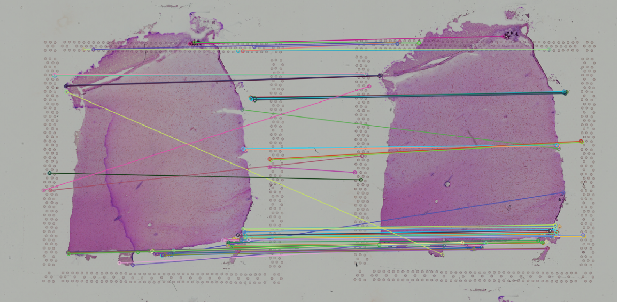
We will make use of the registerSpatialData function to automatically register two Xenium assays onto the Visium assay. The Visium CytAssist image (or the image on the center of the list) would be taken as the image of reference, and hence all other images (or spatial datasets) are to be aligned to the Visium data. Then, registerSpatialData will return a list of VoltRon objects whose assays include both the original and registered versions of spatial coordinates. The shiny app will provide two images for this task:
- An image that shows the matched points across two images, and
- A slideshow with of the reference and registered images that demonstrates the alignment accuracy.
We will select FLANN method for automated alignment which incorporates the SIFT method for automated keypoints selection and utilizes the Fast library for Approximate Nearest Neighbors (FLANN) algorithm for matching keypoints. NOTE: For better alignment performance, users can incorporate image manipulation tools above each image and sync images into the same orientation by rotating, flipping (horizontally and vertically) and negating these images. We always negate DAPI images to align them onto H&E images.
xen_reg <- registerSpatialData(object_list = list(Xen_R1, Vis, Xen_R2))You can save and use the same parameters later, and reproduce the alignment without choosing parameters the second time.
mapping_parameters <- xen_reg$mapping_parameters
xen_reg <- registerSpatialData(object_list = list(Xen_R1, Vis, Xen_R2),
                               mapping_parameters = mapping_parameters)
You can find a presaved set of parameters here.
mapping_parameters <- readRDS("mapping_parameters.rds")
xen_reg <- registerSpatialData(object_list = list(Xen_R1, Vis, Xen_R2),
                               mapping_parameters = mapping_parameters)
If the pre-saved parameters are available, the registration can also be performed without using the shiny app. By using interactive = FALSE, we can register images and VoltRon objects directly.
mapping_parameters <- xen_reg$mapping_parameters
xen_reg <- registerSpatialData(object_list = list(Xen_R1, Vis, Xen_R2),
                               mapping_parameters = mapping_parameters,
                               interactive = FALSE)
In case there are only two images, the first image will be taken as the image of reference. Hence, in order to align the first Xenium Replicate to the Visium dataset, we can create a list of two VoltRon objects as given below.
xen_reg <- registerSpatialData(object_list = list(Vis, Xen_R2))Manual Image Alignment
Given the diverse types of tissue sections and their complex morphology, we need an alternative alignment strategy if automated registration may fail. VoltRon allows manually choosing keypoints (or landmarks) on images that are locations on the tissue with structural/morphological similarity. Similar to the automated mode, the image on the center will be taken as reference and the users will be able to observe the quality of the registration and remove/reselect keypoints as they see fit.
xen_reg <- registerSpatialData(object_list = list(Xen_R1, Vis, Xen_R2))You can save and use the same keypoints later, and reproduce the manual alignment without choosing keypoints for the second time.
mapping_parameters <- xen_reg$mapping_parameters
xen_reg <- registerSpatialData(object_list = list(Xen_R1, Vis, Xen_R2),
                               mapping_parameters = mapping_parameters)
You can find a presaved set of parameters with selected manual keypoints here.
mapping_parameters <- readRDS("mapping_parameters_manual.rds")
xen_reg <- registerSpatialData(object_list = list(Xen_R1, Vis, Xen_R2),
                               mapping_parameters = mapping_parameters)
If the pre-saved keypoints are available with parameters, the registration can also be performed without using the shiny app. By using interactive = FALSE, we can register images and VoltRon objects directly.
mapping_parameters <- xen_reg$mapping_parameters
xen_reg <- registerSpatialData(object_list = list(Xen_R1, Vis, Xen_R2),
                               mapping_parameters = mapping_parameters,
                               interactive = FALSE)
In case there are only two images, the first image will be taken as the image of reference. Hence, in order to align the first Xenium Replicate to the Visium dataset. We can create a list of two VoltRon objects as given below.
xen_reg <- registerSpatialData(object_list = list(Vis, Xen_R2))Combine VoltRon object
Now that the VoltRon objects of Xenium and Visium datasets are accurately aligned, we can combine these objects to create one VoltRon object with three layers. Since all sections are derived from the same tissue block, we want them to be associated with the same sample, hence we define the sample name as well. VoltRon will recognize that all layers are originated from the same sample/block, and choose the majority assay as the main assay.
merge_list <- xen_reg$registered_spat
VRBlock <- merge(merge_list[[1]], merge_list[-1], samples = "10XBlock")
VRBlock
10XBlock:
Layers: Section1 Section2 Section3
Assays: Xenium(Main) Visium
Features: RNA(Main) Here, we can quickly check the change in spatial coordinate systems
in the new tissue block. The registerSpatialData function
synchronizes the coordinate systems of all VoltRon objects in the list
before merging. Both Xenium sections have now two coordinate system
where the registered system main_reg is the default
one.
vrSpatialNames(VRBlock, assay = "all") Assay Layer Sample Spatial Main
Assay1 Xenium Section1 10XBlock main,main_reg main_reg
Assay2 Visium Section2 10XBlock main main
Assay3 Xenium Section3 10XBlock main,main_reg main_regData/Label Transfer Across Layers
The combined VoltRon object of Visium and Xenium datasets can be used to transfer information across layers and assays. This is accomplished by aggregating and summarizing, for example, gene counts of cells from the Xenium assay aligned to Visium spots. Either labels or cell types can be summarized to generate:
- pseudo cell type abundance assays or
- pseudo gene expression assays.
Data Transfer (Cells->Spots)
We must first determine the names of the assays where labels are transfered from one to the other. For the sake of this tutorial, we can select Assay1 of Xenium as the source assay and the Assay2 of Visium as the destination assay.
SampleMetadata(VRBlock) Assay Layer Sample
Assay1 Xenium Section1 10XBlock
Assay2 Visium Section2 10XBlock
Assay3 Xenium Section3 10XBlockThe transferData function detects the types of both the source (from) and the destination (to) assays and determines the how the data should be transfered. We can first transfer data from the Xenium assay to the Visium assay (hence Cells -> Spots), the raw count data of each cell in the source Xenium assay will be aggregated into spots in a new count feature data type in the Visium assay. The new feature data with aggregated counts will be named RNA_pseudo.
VRBlock <- transferData(VRBlock, from = "Assay1", to = "Assay2")VoltRon supports multiple feature type within each assay. Now, the Visium assay includes two spot-type features:
- the original Visium spot feature counts,
- a pseudo Visium feature count matrix with aggregated Xenium raw counts.
vrMainAssay(VRBlock) <- "Visium"
VRBlock
VoltRon Object
10XBlock:
Layers: Section1 Section2 Section3
Assays: Visium(Main) Xenium
Features: RNA(Main) RNA_pseudo We can now visualize both the original and aggregated counts of a gene, such as ERBB2 and ESR1 that marks ductal carcinoma in situ (DCIS) regions, to validate the correlation of gene signatures across adjacent tissue sections, and to validate the accuracy of the automated image alignment. Here, PGR is also expressed at a small DCIS region found on adipocyte niche of the tissue.
library(patchwork)
vrMainFeatureType(VRBlock, assay = "Visium") <- "RNA"
g1 <- vrSpatialFeaturePlot(VRBlock,
                           features = c("ERBB2", "ESR1", "PGR"), crop = FALSE,
                           norm = FALSE, ncol = 3)
vrMainFeatureType(VRBlock, assay = "Visium") <- "RNA_pseudo"
g2 <- vrSpatialFeaturePlot(VRBlock,
                           features = c("ERBB2", "ESR1", "PGR"), crop = FALSE,
                           norm = FALSE, ncol = 3)
g1 / g2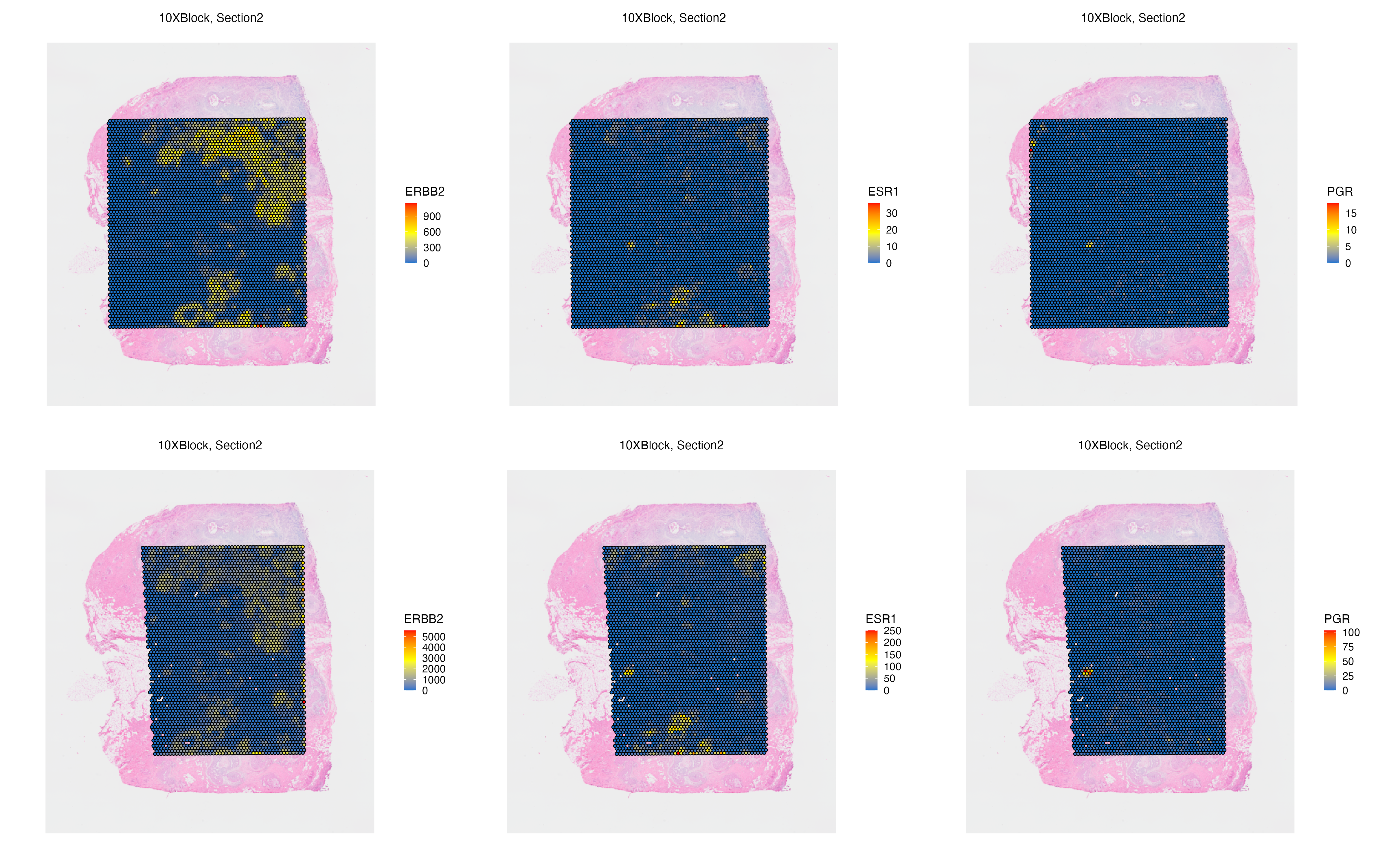
Data Transfer (Spots->Cells)
A similar transfer can be achieved in the opposite direction. We can select Assay2 of Visium as the source assay and Assay1 of Xenium as the destination, thus we can transfer whole transcriptome counts of the Visium assays to Xenium to create new feature sets for Xenium data with more features originally available in the Xenium panel.
vrMainFeatureType(VRBlock, assay = "Visium") <- "RNA"
VRBlock <- transferData(VRBlock, from = "Assay2", to = "Assay1")
We now set the main feature set of the Xenium assays.
vrMainFeatureType(VRBlock, assay = "Xenium") <- "RNA_pseudo"
vrMainFeatureType(VRBlock, assay = "all")
Assay Feature
1 Assay1 RNA_pseudo
2 Assay2 RNA
3 Assay3 RNAlibrary(patchwork)
g1 <- vrSpatialFeaturePlot(VRBlock,
assay = "Assay1", features = c("ERBB2", "ESR1", "PGR"),
crop = TRUE, norm = FALSE, alpha = 1, n.tile = 300, ncol = 3)
g2 <- vrSpatialFeaturePlot(VRBlock,
assay = "Assay2", features = c("ERBB2", "ESR1", "PGR"),
crop = TRUE, norm = FALSE, alpha = 1, ncol = 3)
g1 / g2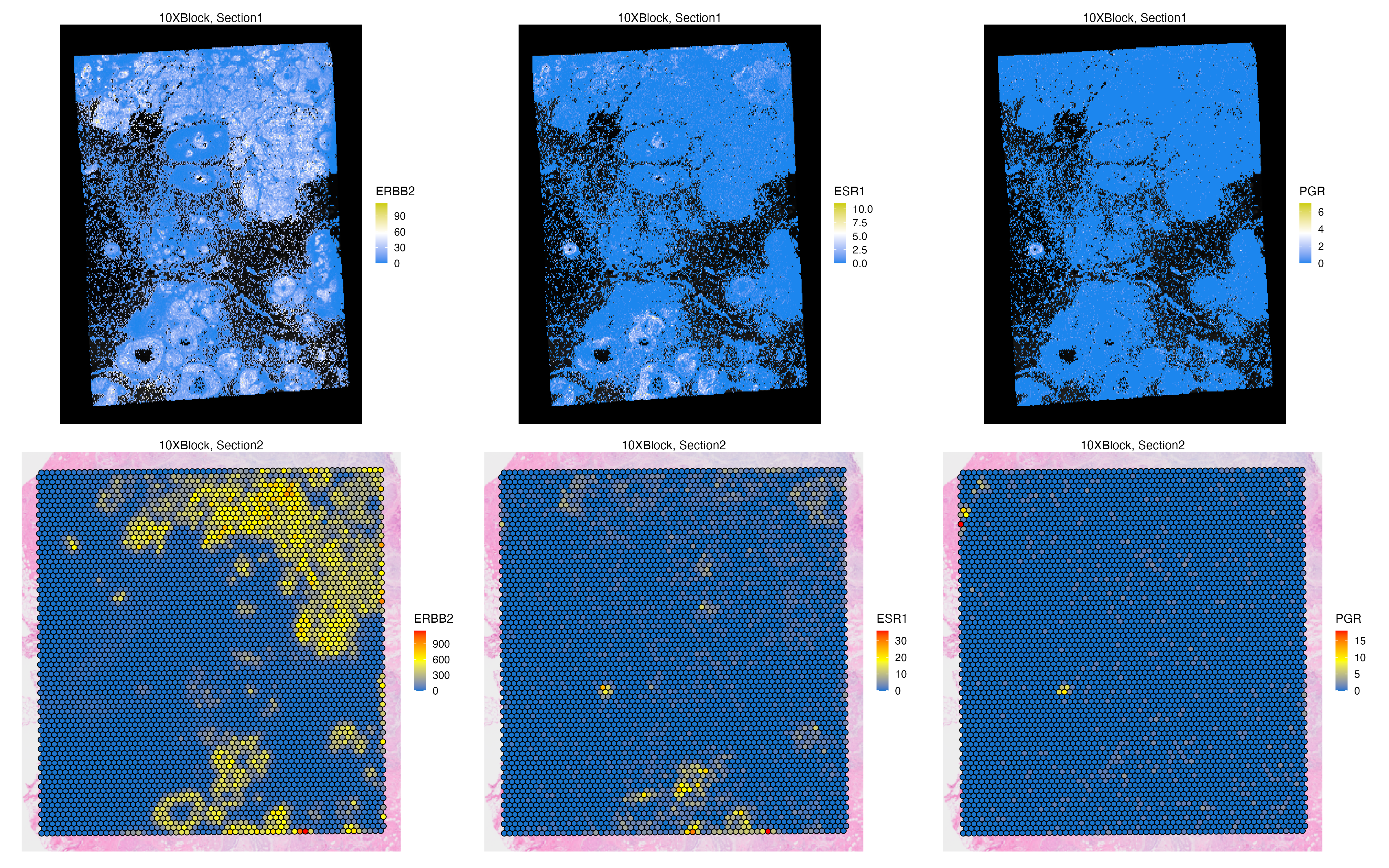
Label Transfer (Cells->Spots)
The transferData function can also transfer metadata features across layers and assays. In this case, we will transfer cell type labels that were trained on the Xenium sections onto the Visium sections. We will use the cluster labels generated at the end of the Xenium analysis section of workflow from Cell/Spot Analysis. You can download the VoltRon object with clustered and annotated Xenium cells along with the Visium assay from here.
VRBlock <- readRDS("VRBlock_data_clustered.rds")
vrSpatialPlot(VRBlock, assay = "Xenium", group.by = "CellType", pt.size = 0.4)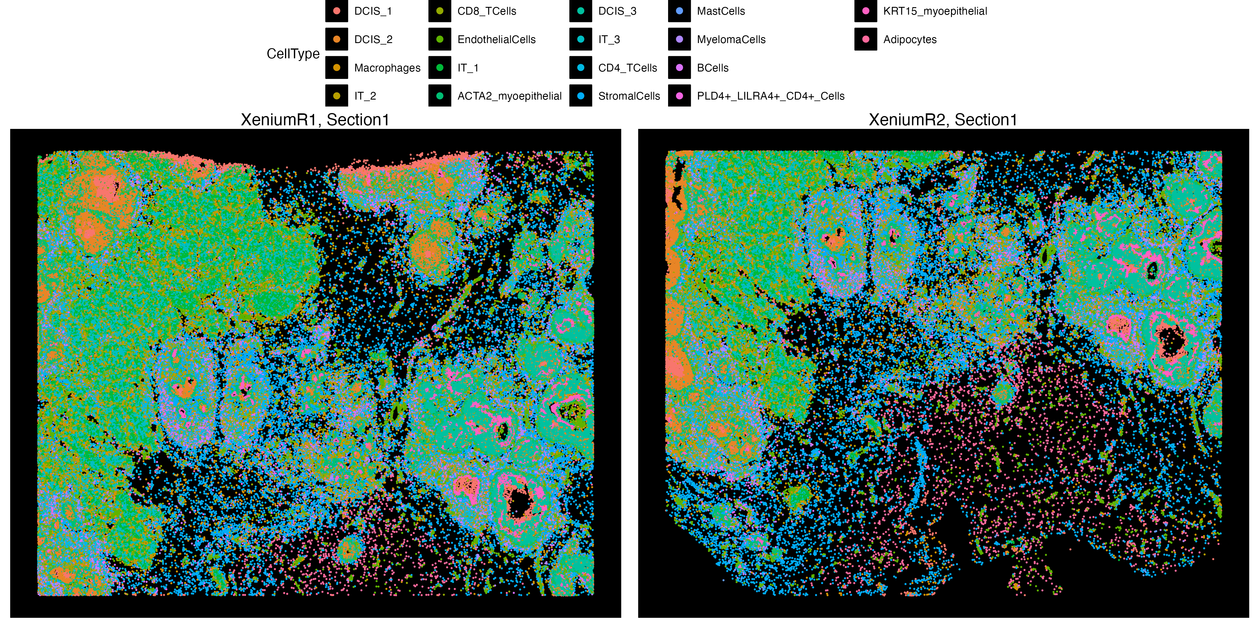
Here, we can see that both Xenium layers are clustered and annotated where we can use these cell annotations and transfer them to the Visium assay to create a new feature data of estimated cell type abundances. If the features argument is specified, and if its a single metadata feature with, e.g. cell types, then the each spot at the new pseudo Visium will be collection of abundances of the categories within that metadata feature.
VRBlock <- transferData(VRBlock, from = "Assay1", to = "Assay2", features = "CellType",
                        new_feature_name = "Visium_CellType")
vrMainAssay(VRBlock) <- "Visium"
VRBlock
VoltRon Object
10XBlock:
Layers: Section1 Section2 Section3
Assays: Visium(Main) Xenium
Features: RNA(Main) Visium_CellType By visualizing the transferred labels on the Visium spots, we can see abundance of some DCIS and invasive tumor subtypes.
vrMainFeatureType(VRBlock) <- "Visium_CellType"
vrSpatialFeaturePlot(VRBlock, assay = "Visium",
                     features = c("IT_1","DCIS_2"),
                     crop = TRUE, alpha = 1, ncol = 3)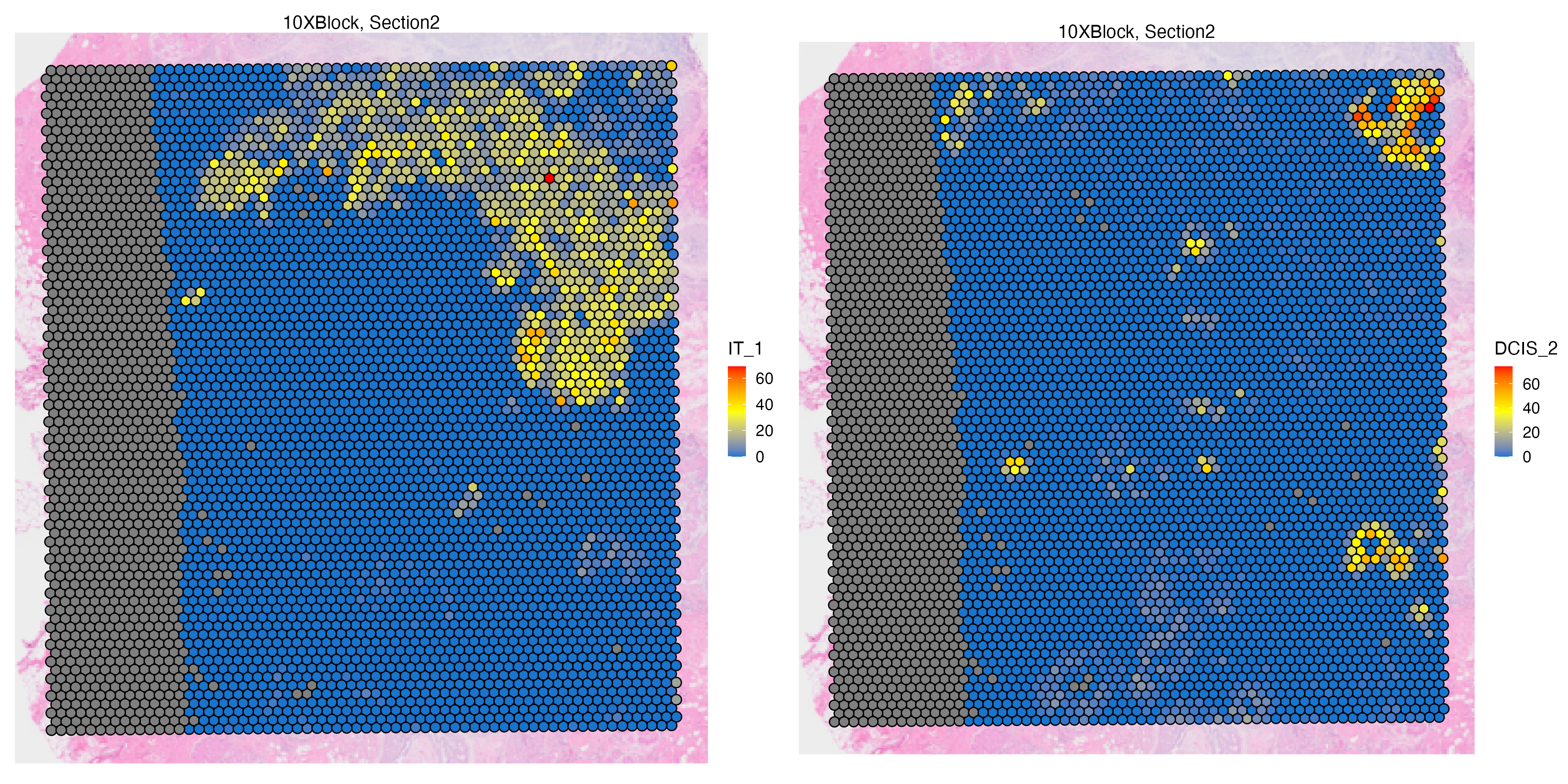
Label Transfer (ROIs->…)
VoltRon allows users to annotate regions of interests (ROIs) in a given assay and transfer the annotations to these ROIs across other assays within the same tissue block. Let us annotate two specific tumor regions in the Visium section. In the process, a new assay called ROIAnnotation will be added to the VoltRon object.
VRBlock <- annotateSpatialData(VRBlock, assay = "Visium",
                               label = "annotation", use.image.only = TRUE)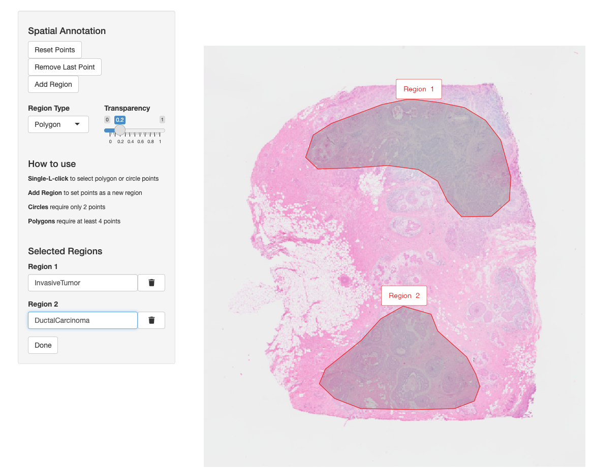
You can observe the changes in the object and check the assay ID of
this new ROI type assay using SampleMetadata function.
vrMainAssay(VRBlock) <- "Xenium"
VRBlock
VoltRon Object
10XBlock:
Layers: Section1 Section2 Section3
Assays: Xenium(Main) Visium ROIAnnotation
Features: RNA(Main) SampleMetadata(VRBlock) Assay Layer Sample
Assay1 Xenium Section1 10XBlock
Assay2 Visium Section2 10XBlock
Assay3 Xenium Section3 10XBlock
Assay4 ROIAnnotation Section2 10XBlockThe metadata of the ROI assay will include the annotation of the ROIs as well.
Metadata(VRBlock, assay = "ROIAnnotation") Assay Layer Sample annotation
InvasiveTumor_Assay4 ROIAnnotation Section2 10XBlock InvasiveTumor
DuctalCarcinoma_Assay4 ROIAnnotation Section2 10XBlock DuctalCarcinomaNow we can transfer the ROI labels from the annotation metadata column and define the same metadata column in the remaining assays.
VRBlock <- transferData(object = VRBlock, from = "Assay4", to = "Assay1",
features = "annotation")
VRBlock <- transferData(object = VRBlock, from = "Assay4", to = "Assay3",
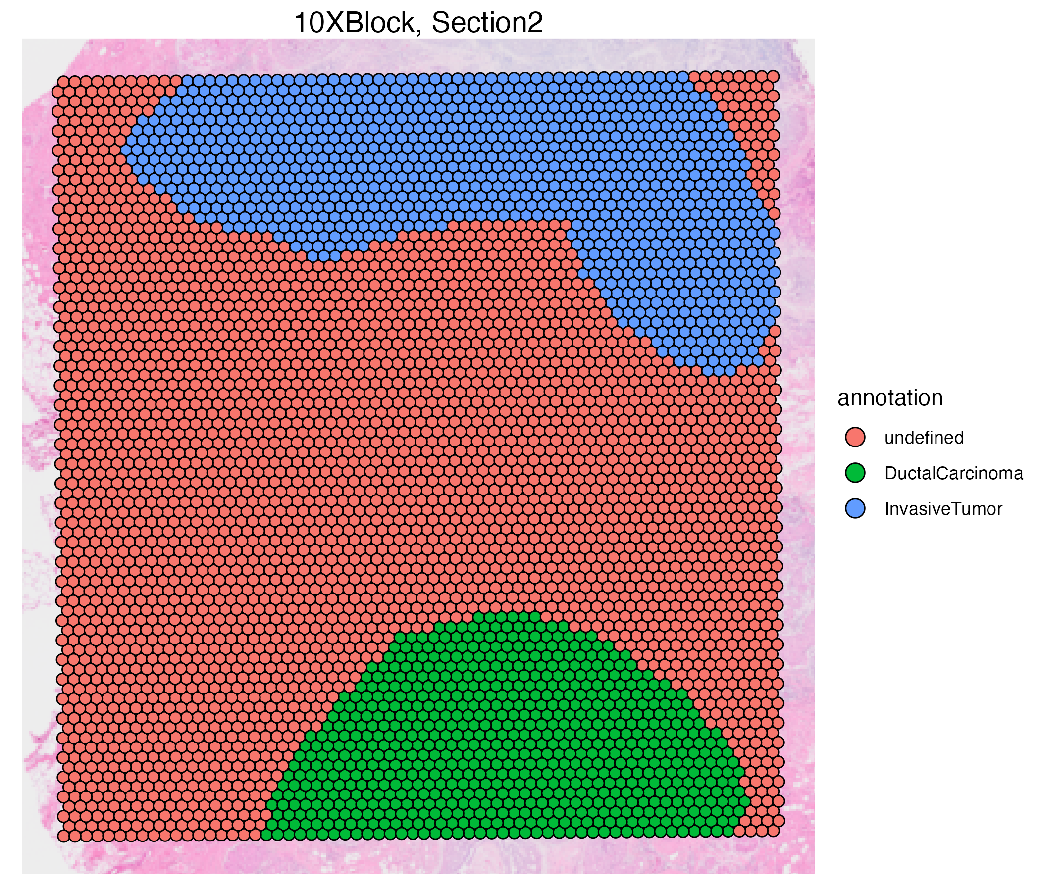
features = "annotation")Let us observe the changes across all assays.
vrSpatialPlot(VRBlock, group.by = "annotation", assay = "Xenium", crop = TRUE)
vrSpatialPlot(VRBlock, group.by = "annotation", assay = "Visium", crop = TRUE)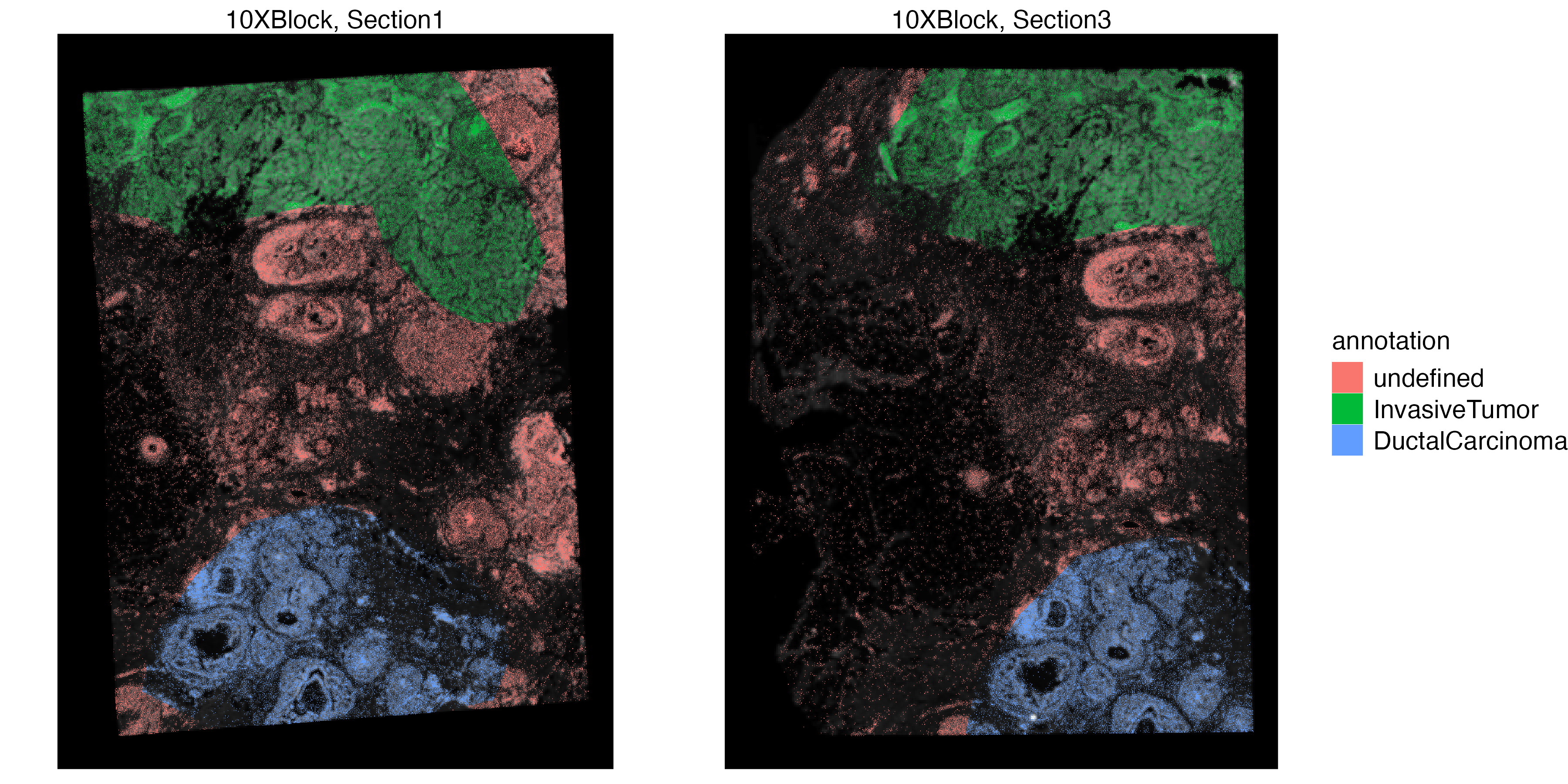
You can also use the addSpatialLayer function to overlay annotation segments to the spatial plot of the Xenium data.
if(!requireNamespace("ggnewscale"))
  install.packages("ggnewscale")
vrSpatialPlot(VRBlock, group.by = "CellType", assay = "Assay1", crop = TRUE) |>
  addSpatialLayer(VRBlock, assay = "ROIAnnotation", group.by = "annotation", spatial = "main", alpha = 0.4)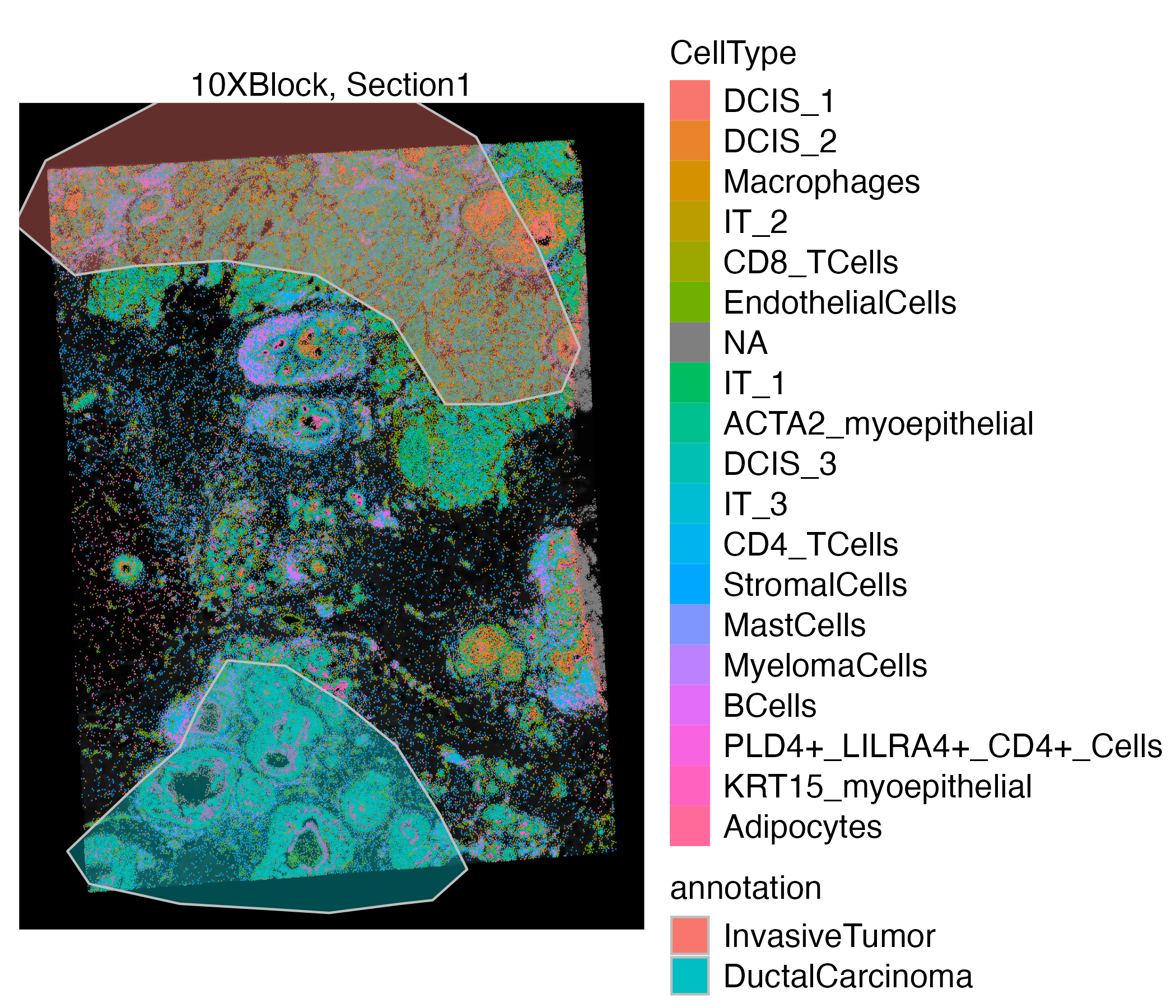
Alignment of Xenium and H&E
In this use case, we will align immunofluorescence (IF) of the Xenium In Situ platform to an H&E images generated from the same sections as the Xenium. VoltRon provides built-in utilities to import images as spatial datasets where tiles are the spatial points. We will import both Xenium and H&E images into two separate VoltRon objects and overlay H&E images.
You can download the Xenium readout and the H&E image of the same tissue section from the 10x Genomics website (specifically, import In Situ Replicate 1 and Supplemental: Post-Xenium H&E image (TIFF)).
# dependencies
if(!requireNamespace("RBioFormats"))
BiocManager::install("RBioFormats")
if(!requireNamespace("arrow"))
install.packages("arrow")
if(!requireNamespace("rhdf5"))
BiocManager::install("rhdf5")
library(VoltRon)
# import Xenium
Xen_R1 <- importXenium("Xenium_R1/outs", sample_name = "XeniumR1",
resolution_level = 3,
overwrite_resolution = TRUE)
# import H&E image
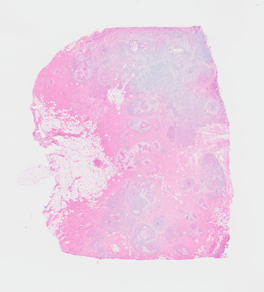
Xen_R1_image <- importImageData("Xenium_FFPE_Human_Breast_Cancer_Rep1_he_image.tif",
sample_name = "XeniumR1image",
channels = "H&E")
Xen_R1_imageVoltRon Object
XeniumR1image:
Layers: Section1
Assays: ImageData(Main) Let’s take a look at the image of the Xen_R1_image object. We use the scale.perc argument to scale down the image for faster rendering.
vrImages(Xen_R1_image, scale.perc = 5)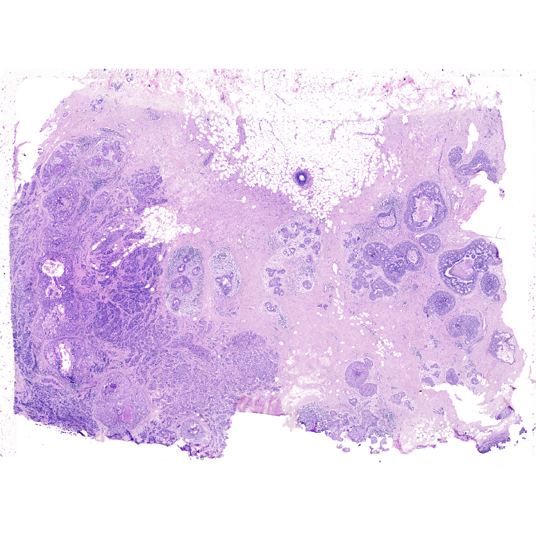
Automated Image Alignment
We can use the registerSpatialData function to warp/align images across multiple VoltRon objects and define these aligned images additional channels of existing coordinate systems of assays in one of these VoltRon objects.
First we align the H&E image to the DAPI image of the Xenium replicate. Similar to the first use case, we need to negate the DAPI image and rotate the image to match its perspective to the H&E image. We can also scale the resolution of the H&E image to 9103.71x6768.63 in order to speed up the registration, however the original scales can also be used.
xen_reg <- registerSpatialData(object_list = list(Xen_R1, Xen_R1_image))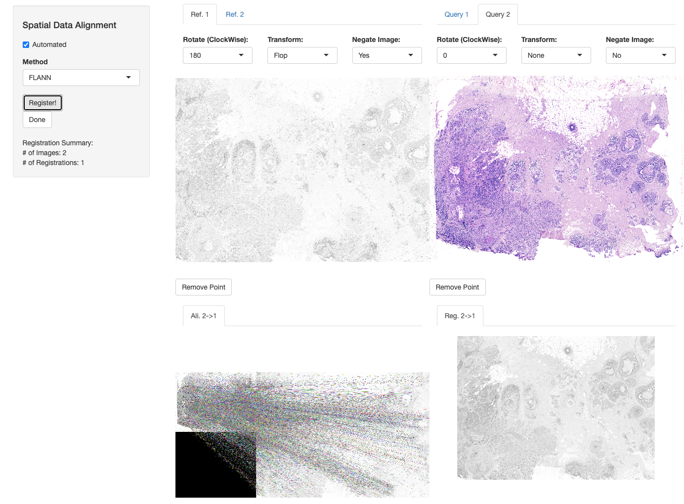
Now we create a new channel for the existing coordinate system of the Xenium data. Here, the spatial key of the registered H&E image will be main_reg. We choose the destination of the registered image which is the first Assay of the Xenium data (i.e. Assay1). The original DAPI coordinate system, and we give a name for the new image/channel which is H&E.
Xen_R1_image_reg <- xen_reg$registered_spat[[2]]
vrImages(Xen_R1[["Assay1"]], channel = "H&E") <- vrImages(Xen_R1_image_reg, name = "main_reg", channel = "H&E")
We can now observe the new channels (H&E) available for the Xenium assay using vrImageChannelNames.
vrImageChannelNames(Xen_R1) Assay Layer Sample Spatial Channels
Assay1 Xenium Section1 XeniumR1 main DAPI,H&EWe can call the registered H&E image of the Xenium data or later put the aligned H&E when calling vrSpatialPlot or vrSpatialFeaturePlot.
vrImages(Xen_R1, channel = "H&E", scale.perc = 5)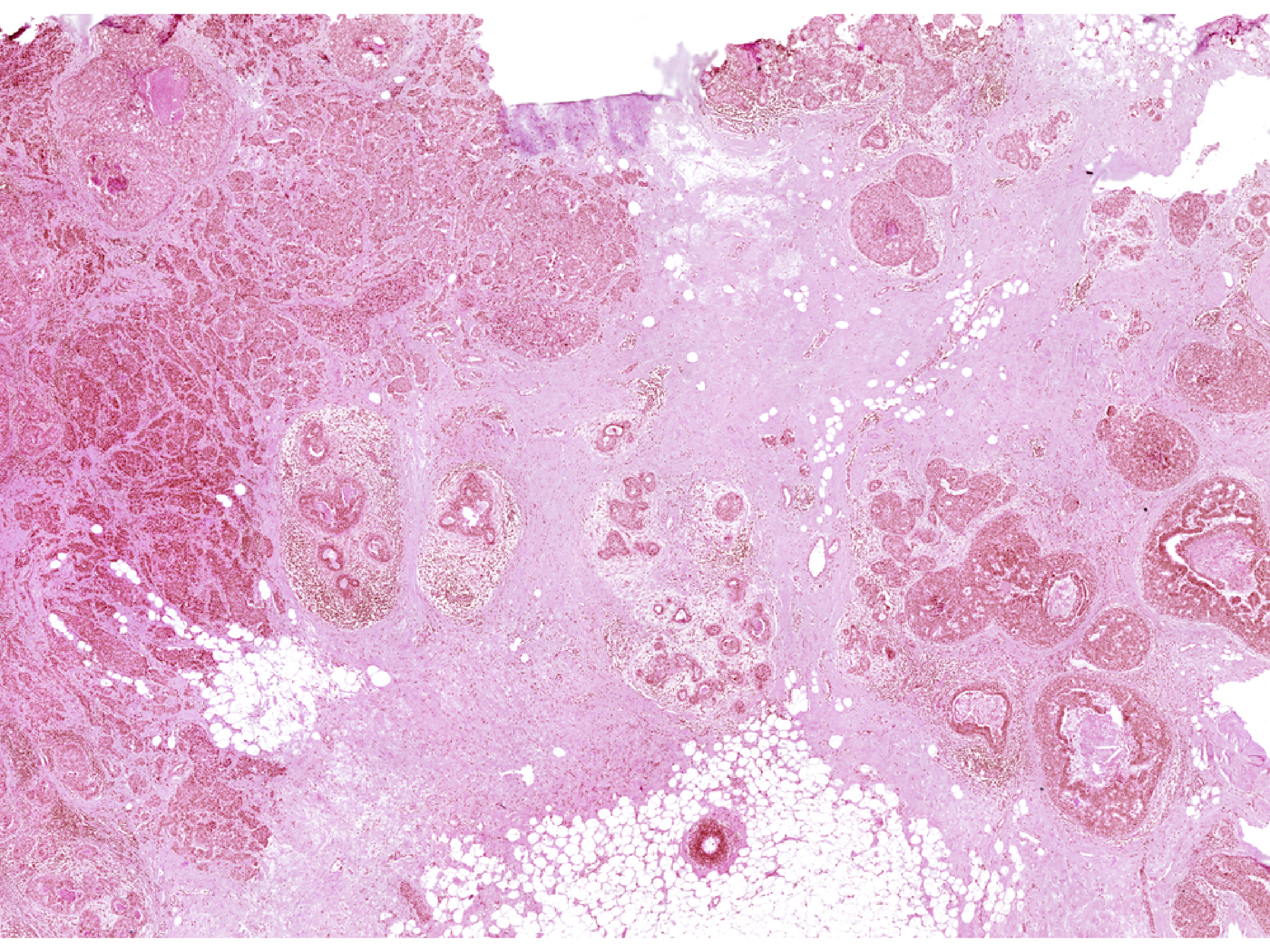
Non-Rigid Alignment
VoltRon allows performing non-rigid image registration and spatial data alignment using the SimpleITK’s C++ library. With SimpleITK, we conduct a coarse-to-fine alignment workflow where we first perform a global alignment using FLANN or BRUTE-FORCE methods, and then perform a fine alignment using SimpleITK. We first use either affine or homography transformation and then interpolate images, points and segments using B-spline method.
To facilitate non-rigid alignment, we require to install the SimpleITK package as below:
install.packages("path/to/SimpleITK_2.5.3.tgz", repos = NULL, type = "binary")or if you are not using MacOS-arm or Windows, please build SimpleITK from source with Elastix module enabled. Please note that the building process may take a while.
if (!require("devtools", quietly = TRUE))
    install.packages("devtools")
devtools::install_github(
  repo = "SimpleITK/SimpleITKRInstaller",
  configure.vars=c("MAKEJ=6",
                   "ADDITIONAL_SITK_MODULES=-DSimpleITK_USE_ELASTIX=ON"))
We can then use registerSpatialData function as before and select “Affine + Non-Rigid” and “BSpline (SimpleITK)” options to conduct non-rigid alignment.
library(SimpleITK)
xen_reg <- registerSpatialData(object_list = list(Xen_R1, Xen_R1_image))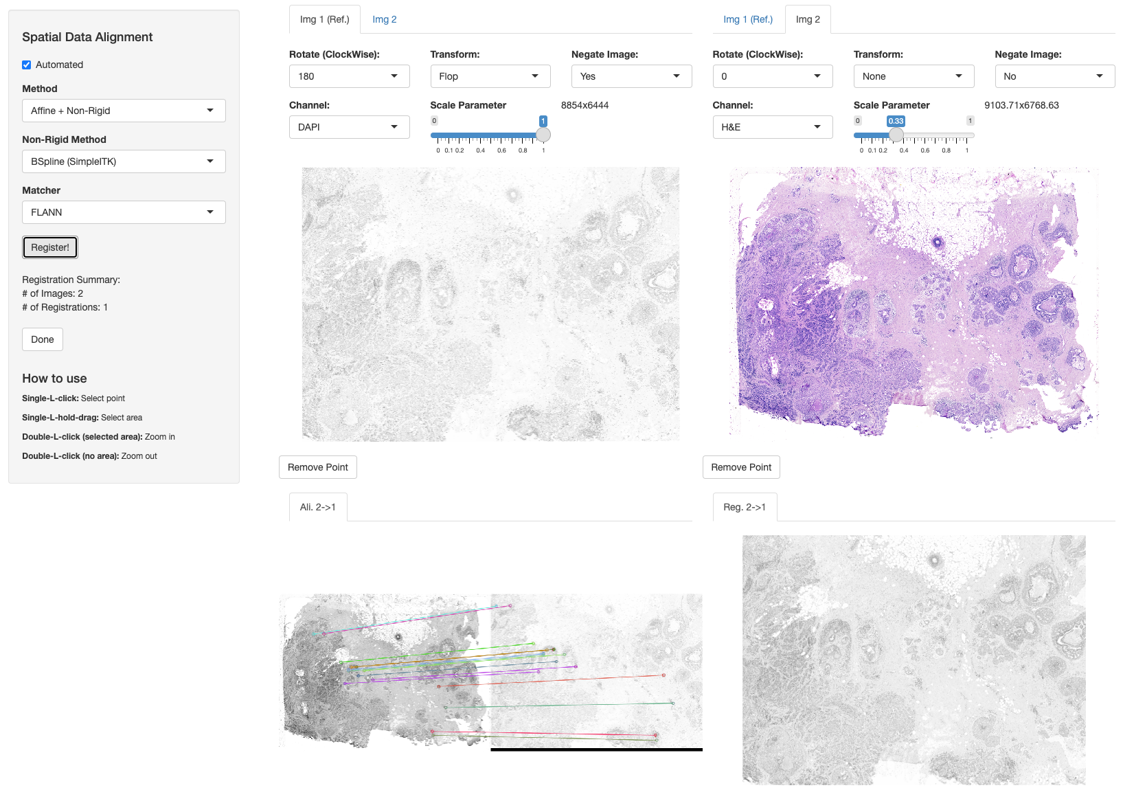
Alignment of Visium and Visium
In the next use case, we will align H&E images associated with Visium data generated from tissue block sections of adult humans with postmortem dorsolateral prefrontal cortex (DLPFC). Two pairs of adjacent sections were obtained from the tissue block of the third donor. Each pair are composed of two 10 \(\mu\)m serial tissue sections, and pairs are located 300 \(\mu\)m apart from each other. Hence, we align each pair individually. The datasets can be downloaded from here.
# dependencies
if(!requireNamespace("rhdf5"))
  BiocManager::install("rhdf5")

# import Visium data
library(VoltRon)
DLPFC_1 <- importVisium("DLPFC/151673", sample_name = "DLPFC_1")
DLPFC_2 <- importVisium("DLPFC/151674", sample_name = "DLPFC_2")
DLPFC_3 <- importVisium("DLPFC/151675", sample_name = "DLPFC_3")
DLPFC_4 <- importVisium("DLPFC/151676", sample_name = "DLPFC_4")
Automated Image Alignment
We will again use the registerSpatialData function to automatically register two Visium assays (two H&E images). This time, we will use the BRUTE-FORCE method for automated alignment which we found to be more accurate compared to FLANN when aligning two H&E images. The shiny app also provides two tuning parameters that used by the BRUTE-FORCE workflow:
- # of Features option specifies the number of maximum image features spotted within each image which later be used to match to the other image.
- Match % specifies the percentage of these features matching at max which in turn used to compute the registration/transformation matrix.
We will use 1000 features for this alignment, set Match % to 20% of the features to be matched across images. The quality of the alignment will be determined by the fine tuning of these parameters where users will immediately observe the alignment quality looking at the slideshow.
DLPFC_list <- list(DLPFC_1, DLPFC_2)
reg1and2 <- registerSpatialData(object_list = DLPFC_list)We can now apply a similar alignment across the second pair of VoltRon objects. We will use 800 features for this alignment, set Match % to 50% of the features to be matched across images.
DLPFC_list <- list(DLPFC_3, DLPFC_4)
reg3and4 <- registerSpatialData(object_list = DLPFC_list)
We can now combine all sections into one VoltRon object. There are two pairs of serial tissue sections, but both pairs (thus 4 sections) are from the same tissue block. Hence, we can combine these two lists into one list and merge VoltRon objects even though sections were aligned separately.
merge_list <- c(reg1and2$registered_spat, reg3and4$registered_spat)
SRBlock <- merge(merge_list[[1]], merge_list[-1], samples = "DLPFC_Block")
SRBlock
VoltRon Object
DLPFC_Block:
Layers: Section1 Section2 Section3 Section4
Assays: Visium(Main)
Features: RNA(Main)Now that we have combined registered pairs of adjacent tissue sections, we should define the adjacency of these pairs in the tissue block.
# two pairs of adjacent sections
connectivity <- data.frame(
  c(1,1,3,3),
  c(1,2,3,4)
)
# adjacent sections are 10 micron apart, and pairs 300 micron
zlocation <- c(0, 10, 300, 310)*params$tissue_lowres_scalef

# add connectivity information to the block
SRBlock <- addBlockConnectivity(SRBlock,
                                connectivity = connectivity,
                                zlocation = zlocation,
                                sample = "DLPFC_Block")
The aligned and connected Visium assays of the DLPFC then could be used for 3D spatial analysis, specifically as shown in the Niche Clustering tutorial.