Molecule Analysis
Molecule Analysis
VoltRon is an end-to-end spatial omics analysis package which also supports investigating spatial points in sub-cellular resolution, including those that are based on Fluorescence in situ hybridization where one can spatially locate each individual molecule that are hybridized
In this tutorial, we provide a number of examples where we show how VoltRon manages, analyzes and visualizes molecules as spatial entities whose identities are given in the metadata of a VoltRon object.
Xenium Breast Cancer Data
In this use case, we analyse readouts of the experiments conducted on example tissue sections analysed by the Xenium In Situ platform. Two tissue sections of 5 \(\mu\)m thickness are derived from a single formalin-fixed, paraffin-embedded (FFPE) breast cancer tissue block. More information on the spatial datasets and the study can also be found on the bioRxiv preprint.
You can import these readouts from the 10x Genomics website (specifically, import In Situ Replicate 1/2). Alternatively, you can download a zipped collection of Xenium readouts from here.
Creating VoltRon objects
VoltRon includes built-in functions for converting readouts of Xenium experiments into VoltRon objects. The importXenium function uses files of the readout of a Xenium experiment under the output folder, and forms a VoltRon object.
In this case, the Xenium data includes two assays (in the same layer) where one is the cell segmentation based cell profile data and the other is the pure molecule assay where the identity (gene of origin) of RNA molecules are given. In order to import the molecules, we use import_molecules = TRUE.
# dependencies
if(!requireNamespace("RBioFormats"))
  BiocManager::install("RBioFormats")
if(!requireNamespace("arrow"))
  install.packages("arrow")
if(!requireNamespace("rhdf5"))
  BiocManager::install("rhdf5")

# import Xenium data
library(VoltRon)
Xen_R1 <- importXenium("Xenium_R1/outs", sample_name = "XeniumR1", import_molecules = TRUE)
Xen_R1
VoltRon Object
XeniumR1:
Layers: Section1
Assays: Xenium(Main) Xenium_mol Ondisk Support (Optional)
In order to save space from large amount of data that is generated in a VoltRon object, you can also save the imported VoltRon object to disk and still accomplish analysis on molecule datasets. We use the saveVoltRon function which stores both the cell and the molecule assay on disk.
Xen_R1 <- saveVoltRon(Xen_R1, format = "HDF5VoltRon",
                      output = "Xen_R1/", replace = TRUE)
The disk-backed data can be loaded once saved on disk again
Xen_R1 <- loadVoltRon("Xen_R1/")Spatial Visualization
With vrSpatialPlot, we can visualize Xenium experiments in subcellular context. We first visualize mRNAs of ACTA2, a marker for smooth muscle cell actin, as well as markers that are found in myoepithelial and breast cancer associated tumor cells.
VoltRon incorporates automated rasterization of point (aggregating points into tiles of equal size) if large number of spatial entities are being visualized, and thus speeds up plotting.
vrSpatialPlot(Xen_R1, group.by = "gene", assay = "Xenium_mol",
group.ids = c("ACTA2", "KRT15", "TACSTD2", "CEACAM6"))![]()
We can interactively select a subset of interest within the tissue section and visualize the localization of these transcripts. Here we subset a ductal carcinoma niche, and visualize mRNAs of four genes.
Xen_R1_subset <- subset(Xen_R1, interactive = TRUE)
Xen_R1_subset <- Xen_R1_subset$subsets[[1]]
vrSpatialPlot(Xen_R1_subset, assay = "Xenium_mol", group.by = "gene",
group.ids = c("ACTA2", "KRT15", "TACSTD2", "CEACAM6"), pt.size = 0.2, legend.pt.size = 5)![]()
We can use the n.tile argument to divide the count of selected group.ids (e.g. genes here) into hexagonal bins. We will use this argument to divide the x and y-axis into 200 tiles and aggregate transcript counts from select group.id
vrSpatialPlot(Xen_R1_subset, assay = "Xenium_mol", group.by = "gene",
group.ids = c("ACTA2", "KRT15", "TACSTD2", "CEACAM6"), n.tile = 200)![]()
Xenium COVID-19 Lung Data
Since VoltRon is capable of analyzing localization of sub-cellular entities such as molecules beyond mRNAs, the analysis may also extend to extracellular molecules such as viral RNA. Using Xenium in situ, we locate the open reading frames (ORFs) of genomics and subgenomics RNA of SARS-CoV-2, namely S2_N and S2_orf1ab and analyze their abundances over the COVID-19 infected lung tissue.
Specifically, we analyse readouts of eight tissue microarray (TMA) tissue sections that were fitted into the scan area of a slide loaded on a Xenium in situ instrument. These sections were cut from control and COVID-19 lung tissues of donors categorized based on disease durations (acute and prolonged). You can download the standard Xenium output folder here.
For more information on the TMA blocks, see GSE190732 for more information.
Across these eight TMA core, we investigate a core of acute case which is originated from a lung with extreme number of detected open reading frames of virus molecules. For convenience, we load a VoltRon object where cells are already annotated. You can also find the RDS file here.
vr2_merged_acute1 <- readRDS(file = "acutecase1_annotated.rds")You would see that we have two assays associated with the tissue section, one for the cells and the other for the molecules.
SampleMetadata(vr2_merged_acute1) Assay Layer Sample
Assay7 Xenium Section1 acute case 1
Assay8 Xenium_mol Section1 acute case 1Spatial Visualization
We can visualize individual S2_N and S2_orf1ab by simply switching to Xenium_mol assay given
vrSpatialPlot(vr2_merged_acute1, assay = "Xenium_mol", group.by = "gene",
              group.ids = c("S2_N", "S2_orf1ab"), n.tile = 500)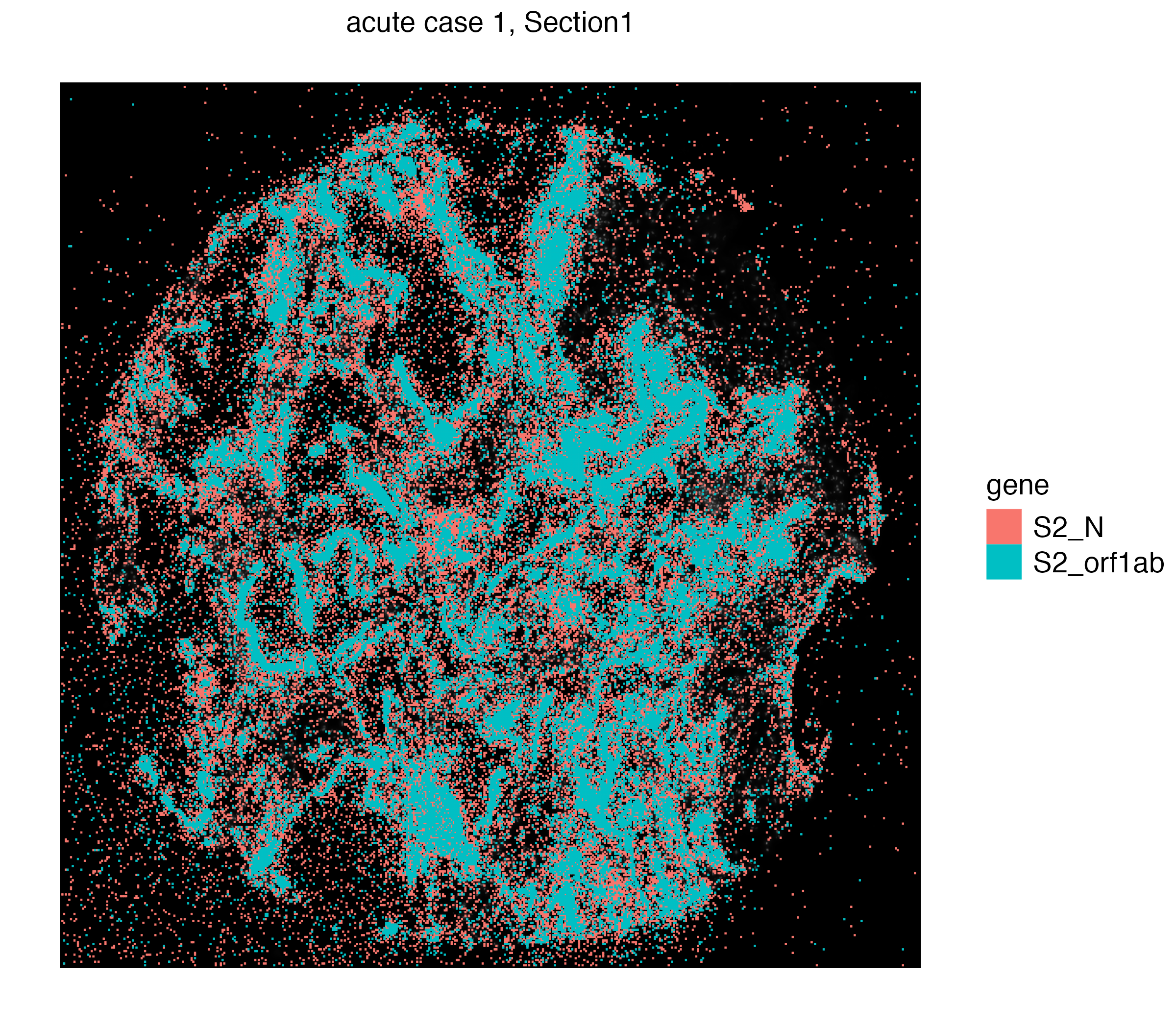
You can also visualize both the cellular and subcellular spatial points on the same plot using addSpatialLayer function, which would show points of the section where virus is abundant with no cell segment on top.
vrSpatialPlot(vr2_merged_acute1, assay = "Xenium_mol", group.by = "gene",
              group.ids = c("S2_N", "S2_orf1ab"), n.tile = 500) |>
  addSpatialLayer(vr2_merged_acute1, assay = "Xenium", group.by = "CellType", plot.segments = TRUE)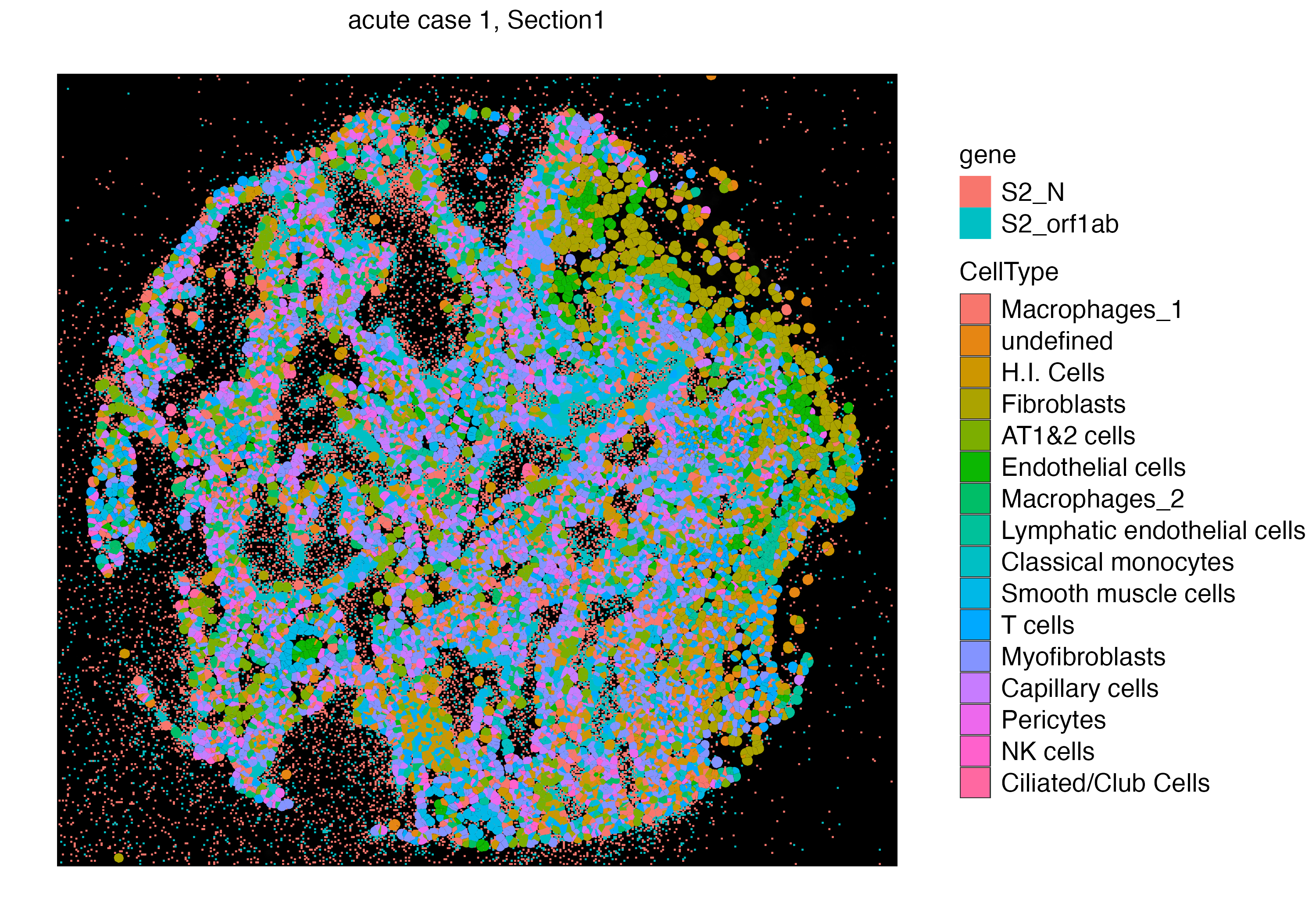
Let us zoom into a specific niche to observe the localization of cell free viral RNA and the surrounding cells.
vr2_merged_acute1_subset <- subset(vr2_merged_acute1, interactive = TRUE)
vr2_merged_acute1_subset <- vr2_merged_acute1_subset$subsets[[1]]
vrSpatialPlot(vr2_merged_acute1_subset, assay = "Xenium_mol", group.by = "gene",
              group.ids = c("S2_N", "S2_orf1ab"), pt.size = 0.4) |>
  addSpatialLayer(vr2_merged_acute1_subset, assay = "Xenium", group.by = "CellType",
                  plot.segments = TRUE, alpha = 0.7)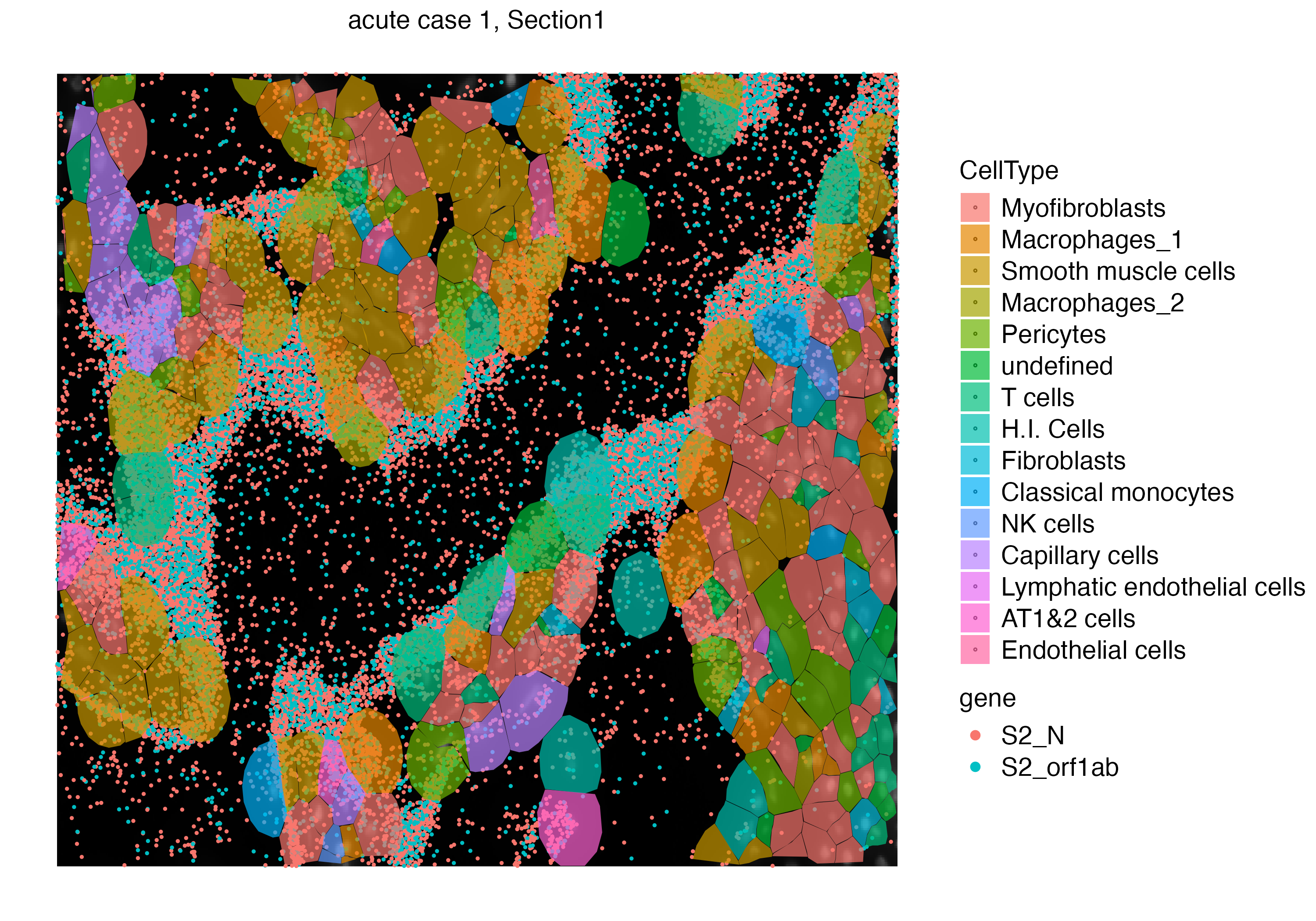
Hot Spot Analysis
Viral RNAs in a highly infected lung sample such as this one may cluster and aggregate in certain niches of the tissue. We can perform hot spot analysis to find these locations of clusters with high abundance (i.e. hot spot) to later identify neighboring cells, and to better understand the effects of the viral infection.
We use the getHotSpotAnalysis function to calculate Getis-Ord statistics for spatial entities, which detects neighborhoods with large values of a feature of interest compared to the global mean of the same feature. Again we are only interested in niches abundant with S2_N and S2_orf1ab molecules.
In case of molecules, we divide the spatial data into tiles of equal size and treat the abundance of molecules as a feature. The neighbors of the tiles are thus other adjacent tiles (eight tiles surrounding each tile). The tiling parameter n.tile can later be changed by the users.
vr2_merged_acute1 <- getHotSpotAnalysis(vr2_merged_acute1, assay = "Xenium_mol",
                                        features = "gene",
                                        group.ids = c("S2_N", "S2_orf1ab"), n.tile = 100)
The getHotSpotAnalysis function will produce test statistics and adjusted p-values for all the selected molecules in the region.
meta <- Metadata(vr2_merged_acute1, assay = "Xenium_mol")
head(meta[meta$gene %in% c("S2_N", "S2_orf1ab"),])
id assay_id overlaps_nucleus gene z_location qv fov_name nucleus_distance
1: 281694020045508_25831b Assay8 0 S2_N 20.37133 40 Q7 402.4913
2: 281694020045511_25831b Assay8 0 S2_N 20.39390 40 Q7 362.9937
3: 281694020042882_25831b Assay8 0 S2_N 20.14611 40 Q7 233.1110
4: 281694020045509_25831b Assay8 0 S2_N 20.14540 40 Q7 241.3636
5: 281694020042883_25831b Assay8 0 S2_N 19.92565 40 Q7 170.5991
6: 281694020042884_25831b Assay8 0 S2_N 19.96041 40 Q7 167.2583
postfix Assay Layer Sample gene_hotspot_stat gene_hotspot_padj gene_hotspot_flag
1: _25831b Xenium_mol Section1 acute case 1 0.000000e+00 1 cold
2: _25831b Xenium_mol Section1 acute case 1 0.000000e+00 1 cold
3: _25831b Xenium_mol Section1 acute case 1 5.752399e-06 1 cold
4: _25831b Xenium_mol Section1 acute case 1 5.752399e-06 1 cold
5: _25831b Xenium_mol Section1 acute case 1 1.150483e-05 1 cold
6: _25831b Xenium_mol Section1 acute case 1 1.150483e-05 1 cold Now we can visualize the localization of S2_N and S2_orf1ab molecules that are located in “hot regions”, or niches that are significantly abundant with these molecules.
vrSpatialPlot(vr2_merged_acute1, assay = "Xenium_mol",
              group.by = "gene_hotspot_flag", group.ids = c("cold", "hot"),
              alpha = 1, colors = list(cold = "blue", hot = "red"),
              background.color = "white")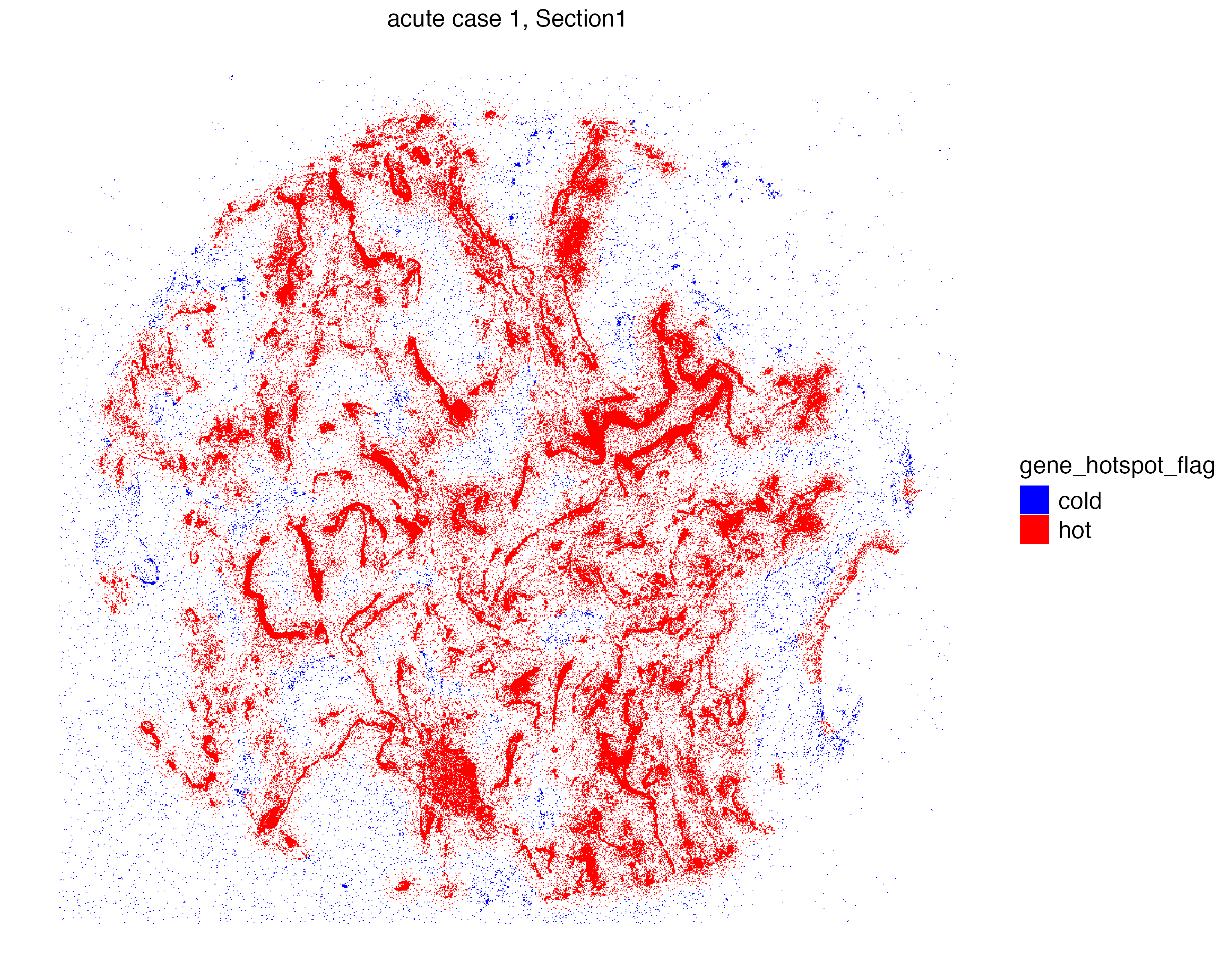
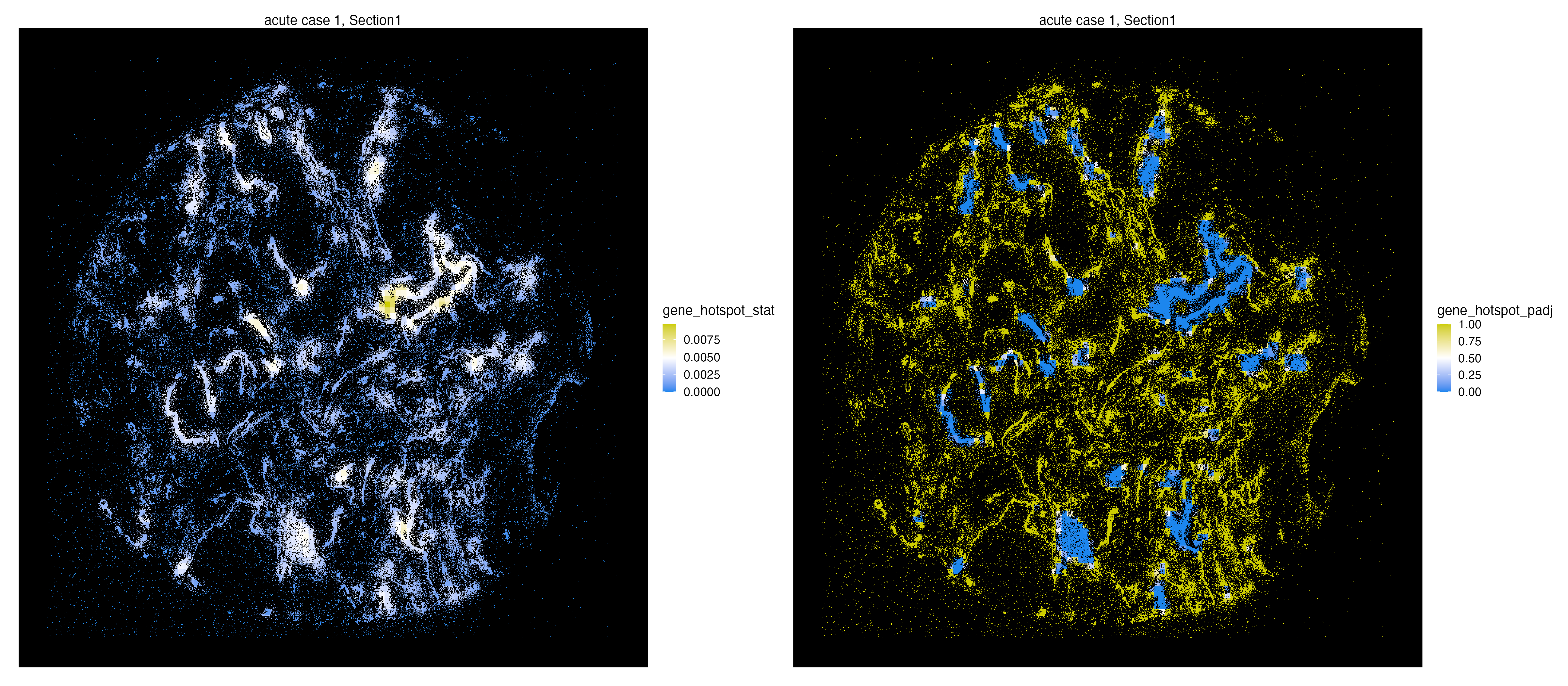
The Getis-Ord test statistics and the associated adjusted p-values are stored within the molecule metadata and can be visualized at will.
library(patchwork)
g1 <- vrSpatialFeaturePlot(vr2_merged_acute1, assay = "Xenium_mol",
                     features = "gene_hotspot_stat",
                     alpha = 1,
                     background.color = "black")
g2 <- vrSpatialFeaturePlot(vr2_merged_acute1, assay = "Xenium_mol",
                     features = "gene_hotspot_padj",
                     alpha = 1,
                     background.color = "black")
g1 | g2