Multi-omics
Multi-omics Analysis
VoltRon is an end-to-end spatial multi-omics platform that enables both automated and manual data alignment workflows to synchronize coordinate frameworks across spatial omics assays. However, upon harmonization of the spatial observations, VoltRon can be used to further transfer and integrate information across omics datasets captured on same and adjacent tissue sections. These assays are not just limited to datasets with single cell and spot resolutions but also to assays solely composed of molecule and image tile observations.
Below, we demonstrate data integration capabilities of VoltRon across distinct modalities using several use cases. In the Spatial Data Alignment, we have highlighted several scenarios to align spatial assays within tissue blocks. However in this tutorial, we demonstrate analysis starting with data alignment and further downstream data integration.
Xenium COVID-19 Lung Data
Xenium in situ platform is compatible with H&E and immunofluorescence imaging , thus researchers can stain whole slides post-Xenium to capture additional information on the morphology of the tissue and integrate it with the Xenium readouts. In this use case, we would like to integrate the post-Xenium H&E image of tissue micro array sections composed of control and COVID-19 lung biopsy punches. Our objective is to assess the localization of SARS‑CoV‑2 virus molecules by integrating pathology image annotations.
VoltRon is capable of analyzing molecule-level subcellular datasets independent of single cells, and specifically those that may also found outside of these cells. The Xenium run was performed with custom Xenium probes designed to hybridize distinct open reading frames of SARS‑CoV‑2 virus molecules. These subcellular entities which then can be detected both within and outside of cells which allows to understand proliferation mechanics of the virus across the tissue. By aligning the image and the associated pathology annotations of the post-Xenium H&E of this slide, we can transfer labels of annotations to Xenium cells and molecules, thus inferring the abundance of viral RNA further.
We analyse readouts of eight tissue micro array (TMA) tissue sections that were fitted into the scan area of a slide loaded on a Xenium in situ instrument. These sections were cut from control and COVID-19 lung tissues of donors categorized based on disease durations (acute and prolonged). You can download the standard Xenium output folder here. For more information on the TMA blocks, please visit GSE190732.
Single Cells and Molecules
Across these eight TMA section, we investigate a section of acute case which is originated from a lung with extreme number of detected open reading frames of virus molecules. For convenience, we load a VoltRon object where cells are already annotated. You can also find the RDS file here.
vr2_merged_acute1 <- readRDS(file = "acutecase1_annotated.rds")Lets visualize both the UMAP and Spatial plot of the annotated cells.
vrEmbeddingPlot(vr2_merged_acute1, assay = "Xenium", embedding = "umap",
                group.by = "CellType", label = TRUE)
vrSpatialPlot(vr2_merged_acute1, assay = "Xenium", group.by = "CellType",
              plot.segments = TRUE)

|

|
We incorporate two open reading frames (ORFs), named S2_N and S2_orf1ab, which represent unreplicated and replicated virus molecules, respectively. We can visualize again tile the count of these virus expressions by specifically selecting these two ORFs.
vrSpatialPlot(vr2_merged_acute1, assay = "Xenium_mol", group.by = "gene",
              group.ids = c("S2_N", "S2_orf1ab"), n.tile = 500)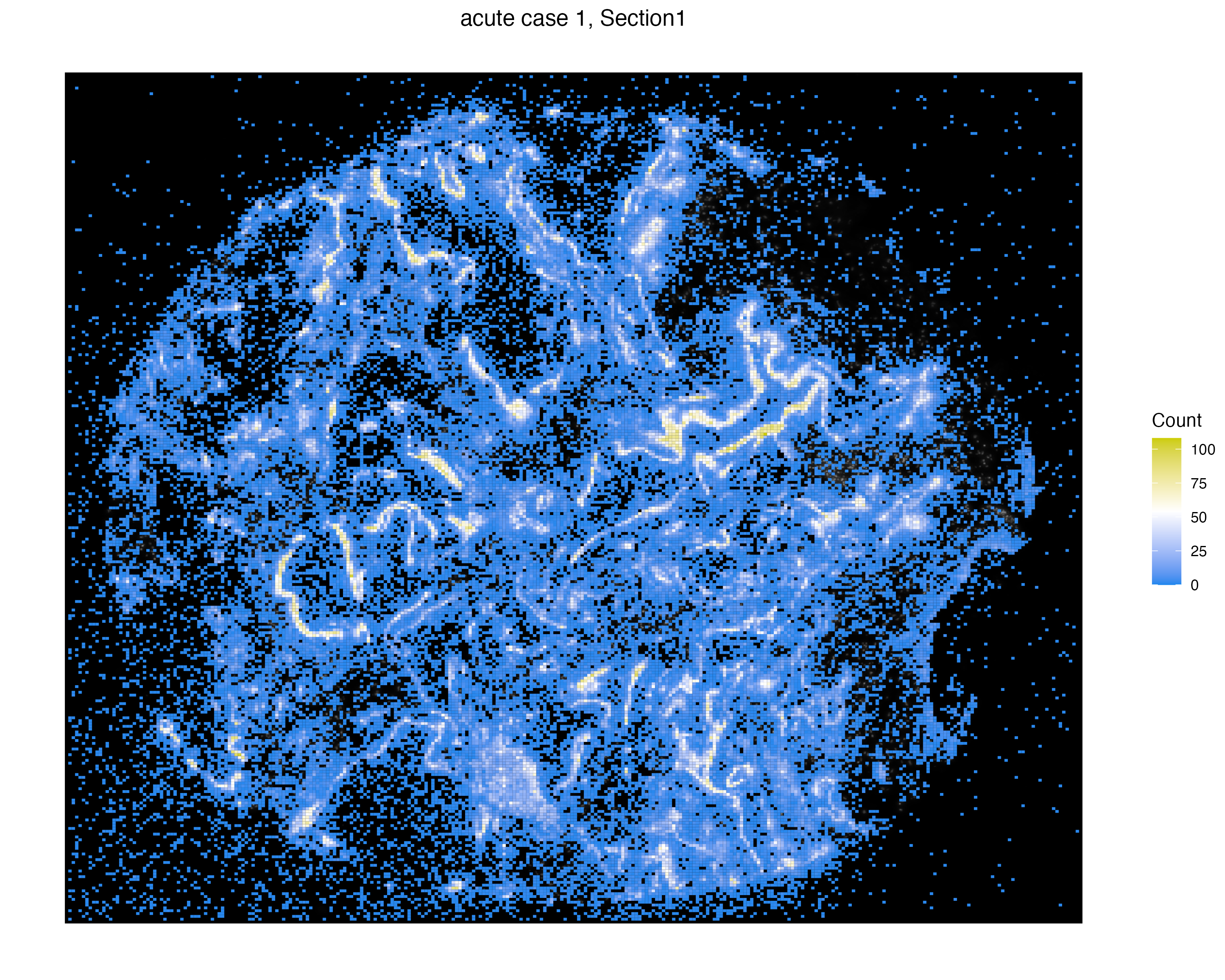
We can even zoom into specific locations at the tissue to investigate virus particles more closely by dropping the n.tile argument and calling interactive visualization.
vrSpatialPlot(vr2_merged_acute1, assay = "Xenium_mol", group.by = "gene",
              group.ids = c("S2_N", "S2_orf1ab"), interactive = TRUE, pt.size = 0.1)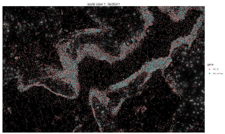
In the following sections, we will integrate pathological images and annotations with Xenium datasets to further understand the spatial localization of virus ORF types over the tissue.
Hot Spot Analysis
VoltRon platform allows users to find hot spots (Regions of increased feature of interest) of several types of spatial entities, for spots, cells, and even molecules. Please see Molecule Analysis Tutorial for more information on hot spot analysis. We switch to the molecule assay of the VoltRon object, and select virus ORFs to detect regions of high viral activity.
vr2_merged_acute1VoltRon Object
acute case 1:
Layers: Section1
Assays: Xenium(Main) Xenium_mol In this case, we are only interested in niches abundant with S2_N and S2_orf1ab molecules. We use the getHotSpotAnalysis function to find regions of high S2_N and S2_orf1ab abundance. The tiling parameter n.tile is necessary to apply Getis-Ord statistics on molecule data since these spatial entities does not have features in a VoltRon object.
vr2_merged_acute1 <- getHotSpotAnalysis(vr2_merged_acute1, assay = "Xenium_mol",
                                        features = "gene",
                                        group.ids = c("S2_N", "S2_orf1ab"), n.tile = 100)
Now we can visualize the localization of molecules that are located in “hot regions”, or niches that are significantly abundant with these molecules.
vrSpatialPlot(vr2_merged_acute1, assay = "Xenium_mol",
              group.by = "gene_hotspot_flag", group.ids = c("cold", "hot"),
              alpha = 1, colors = list(cold = "blue", hot = "red"),
              background.color = "white")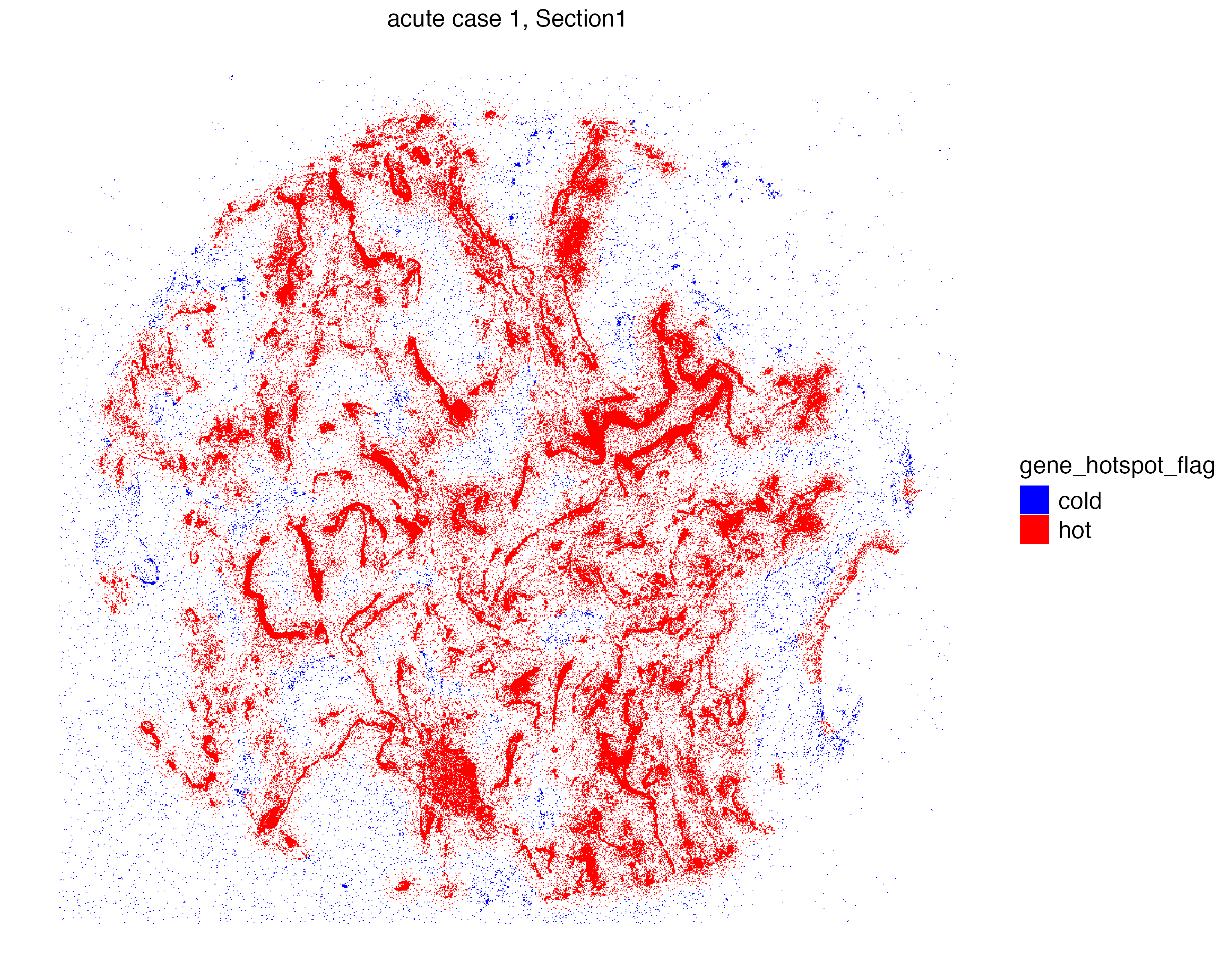
VoltRon allows learning distances between cells and molecules, thus we can calculate the distance between cell types and S2_N and S2_orf1ab molecules aggregated in hot spots which we learned previously using getHotSpotAnalysis.
This is achieved by defining metadata columns for both cell and molecule assays in the getSpatialNeighbors function. We can also choose which molecules are to be used for calculation.
vr2_merged_acute1 <- getSpatialNeighbors(vr2_merged_acute1,
                                         assay = c("Assay7", "Assay8"),
                                         group.by = list(
                                           Assay7 = "CellType",
                                           Assay8 = "gene_hotspot_flag"
                                         ),
                                         group.ids = list(
                                           Assay8 = c("hot")
                                         ),
                                         method = "radius", radius = 20)
We can now visualize the abundance of hot molecules around each cell type. Here we can see that while infected cells (H.I. Cells), T cells and myofibroblasts have considerable amount of surrounding hot spot S2 molecules, fibroblasts and endothelial cells are not.
mat <- igraph::as_adjacency_matrix(vrGraph(vr2_merged_acute1,
                                           assay = c("Assay7", "Assay8")))
mat <- mat[vrSpatialPoints(vr2_merged_acute1, assay = "Assay7"),]
mat <- mat[,vrSpatialPoints(vr2_merged_acute1, assay = "Assay8")]
vr2_merged_acute1$VirusProximity <- rowSums(mat)

# visualize violinplot
vrViolinPlot(vr2_merged_acute1, features = "VirusProximity",
             norm = FALSE, group.by = "CellType")
We can visualize particular cells and molecules simultaneously to observe the distinct localization of these cell types and hot molecules. We use the addSpatialLayer function to overlay these hot spot molecules with a selected set of celltypes from the Xenium assay.
if(!requireNamespace("ggnewscale"))
  install.packages("ggnewscale")
vrSpatialPlot(vr2_merged_acute1, assay = "Xenium", group.by = "CellType",
              group.ids = c("Myofibroblasts", "T cells",
                            "Fibroblasts", "Endothelial cells "),
              plot.segments = TRUE) |>
  addSpatialLayer(vr2_merged_acute1, assay = "Xenium_mol",
                  group.by = "gene_hotspot_flag",
                  group.ids = "hot", colors = list("hot" = "green"))
Automated H&E Registration
VoltRon can analyze and also integrate information from distinct spatial data types such as images, annotations (as regions of interests, i.e. ROIs) and molecules independently. Using such advanced utilities, we can make use of histological information and generate new metadata level information for molecule datasets.
We will first import both histological images and manual annotations using the importImageData function which accepts both images to generate tile/pixel level datasets but also allows one to import either a list of segments or GeoJSON objects for create ROI-level datasets as separate assays in a single VoltRon layer. The .geojson file was generated using QuPath on the same section H&E image of one Xenium section with the acute COVID-19 case. We also have to flip the coordinates of ROI annotations also for they were directly imported from QuPath which incorporates a reverse coordinate system on the y-axis.
Once imported, the resulting VoltRon object will have two assays in a single layer, one for tile dataset of the H&E image and the other for ROI based annotations of again the same image. You can download the H&E image from here, and download the json file from here.
# get image
imgdata <- importImageData("acutecase1_HE.jpg",
                           segments = "acutecase1_membrane.geojson",
                           sample_name = "acute case 1 (HE)")
imgdata <- flipCoordinates(imgdata, assay = "ROIAnnotation")
imgdata
VoltRon Object
acute case 1 (HE):
Layers: Section1
Assays: ImageData(Main) ROIAnnotation
Features: main(Main) By visualizing these annotations interactively, we can see that the ROIs point to the hyaline membranes. Here, we likely find extra-cellular SARS‑CoV‑2 molecules mostly outside of any single cell.
vrSpatialPlot(imgdata, assay = "ROIAnnotation", group.by = "Sample",
              alpha = 0.7, interactive = TRUE)
At a first glance, although the Xenium (DAPI) and H&E images are associated with the same TMA core, they were captured in a different perspective; that is, one image is almost the 90 degree rotated version of the other. We will account for this rotation when we (automatically) align the Xenium data with the H&E image.
vr2_merged_acute1 <- modulateImage(vr2_merged_acute1, brightness = 300, channel = "DAPI")
vrImages(vr2_merged_acute1, assay = "Assay7", scale.perc = 20)
vrImages(imgdata, assay = "Assay1", scale.perc = 20)
We now register the H&E image and annotations to the DAPI image of Xenium section using the registerSpatialData function. We select FLANN (with “Affine” method) automated registration mode, negate the DAPI image of the Xenium slide, turn 90 degrees to the left and set the scale parameter of both images to width = 1859. See Spatial Data Alignment tutorial for more information.
xen_reg <- registerSpatialData(object_list = list(vr2_merged_acute1, imgdata))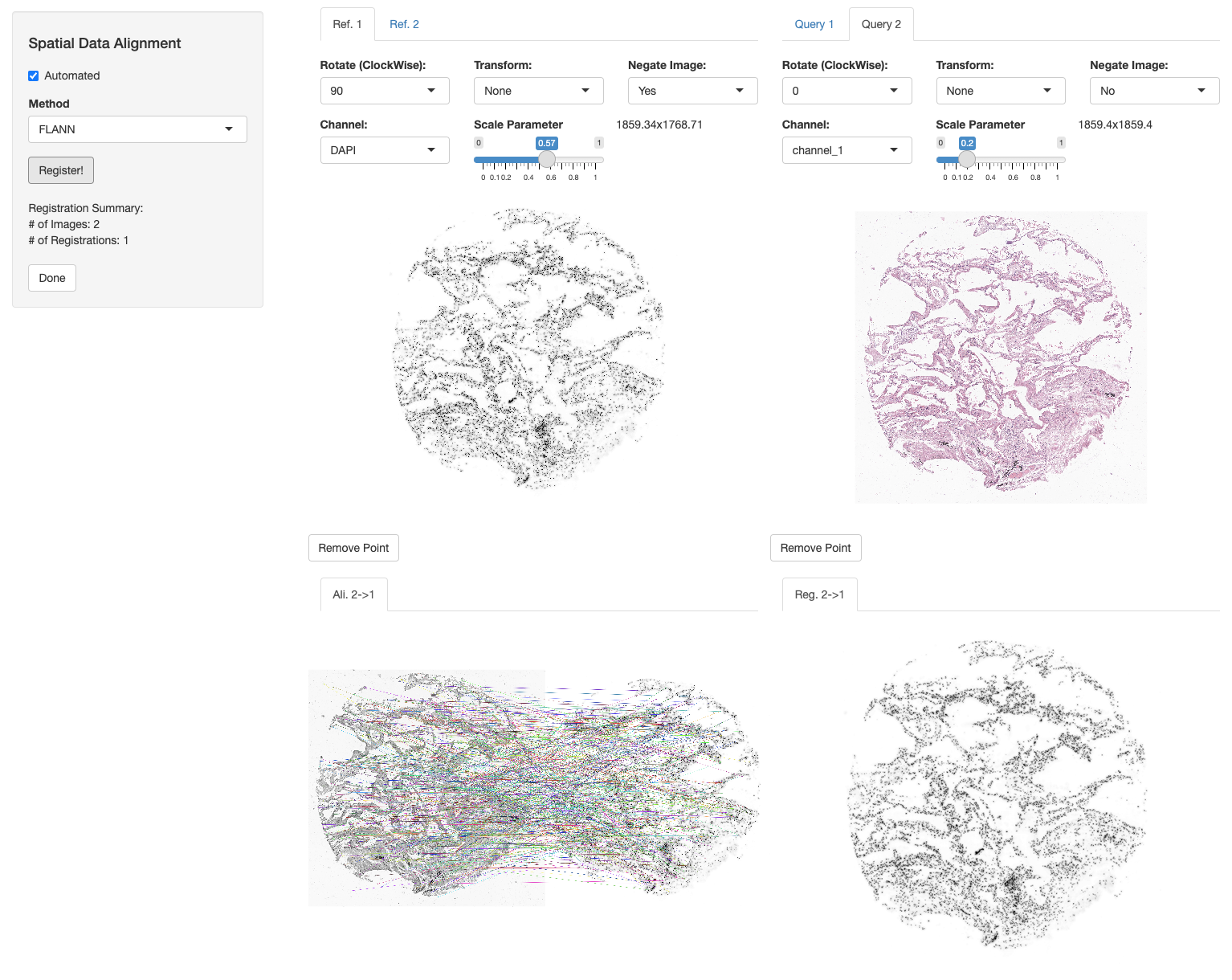
Once registered, we can isolate the registered H&E data and use it further analysis. We can transfer images and their channels across assays of one or multiple VoltRon objects. Here, we save the registered image of the H&E data as an additional channel of Xenium section of the acuse case 1 sample with molecule data.
imgdata_reg <- xen_reg$registered_spat[[2]]
vrImages(vr2_merged_acute1[["Assay7"]], name = "main", channel = "H&E") <-
  vrImages(imgdata_reg, assay = "Assay1", name = "main_reg")
vrImages(vr2_merged_acute1[["Assay8"]], name = "main", channel = "H&E") <-
  vrImages(imgdata_reg, assay = "Assay1", name = "main_reg")
We can now observe the new channels available for the both molecule and cell-level assays of Xenium data.
vrImageChannelNames(vr2_merged_acute1) Assay Layer Sample Spatial Channels
Assay7 Xenium Section1 acute case 1 main DAPI,H&E
Assay8 Xenium_mol Section1 acute case 1 main DAPI,H&EYou can also add the VoltRon object of H&E data as an additional assay of the Xenium section such that one layer includes cell, molecules, ROI Annotations and images in the same time. Specifically, we add the ROI annotation to the Xenium VoltRon object using the addAssay function where we choose the destination sample/block and the layer of the assay.
vr2_merged_acute1 <- addAssay(vr2_merged_acute1,
                              assay = imgdata_reg[["Assay2"]],
                              metadata = Metadata(imgdata_reg, assay = "ROIAnnotation"),
                              assay_name = "ROIAnnotation",
                              sample = "acute case 1", layer = "Section1")
vr2_merged_acute1
VoltRon Object
acute case 1:
Layers: Section1
Assays: ROIAnnotation(Main) Xenium_mol Xenium Interactive Visualization
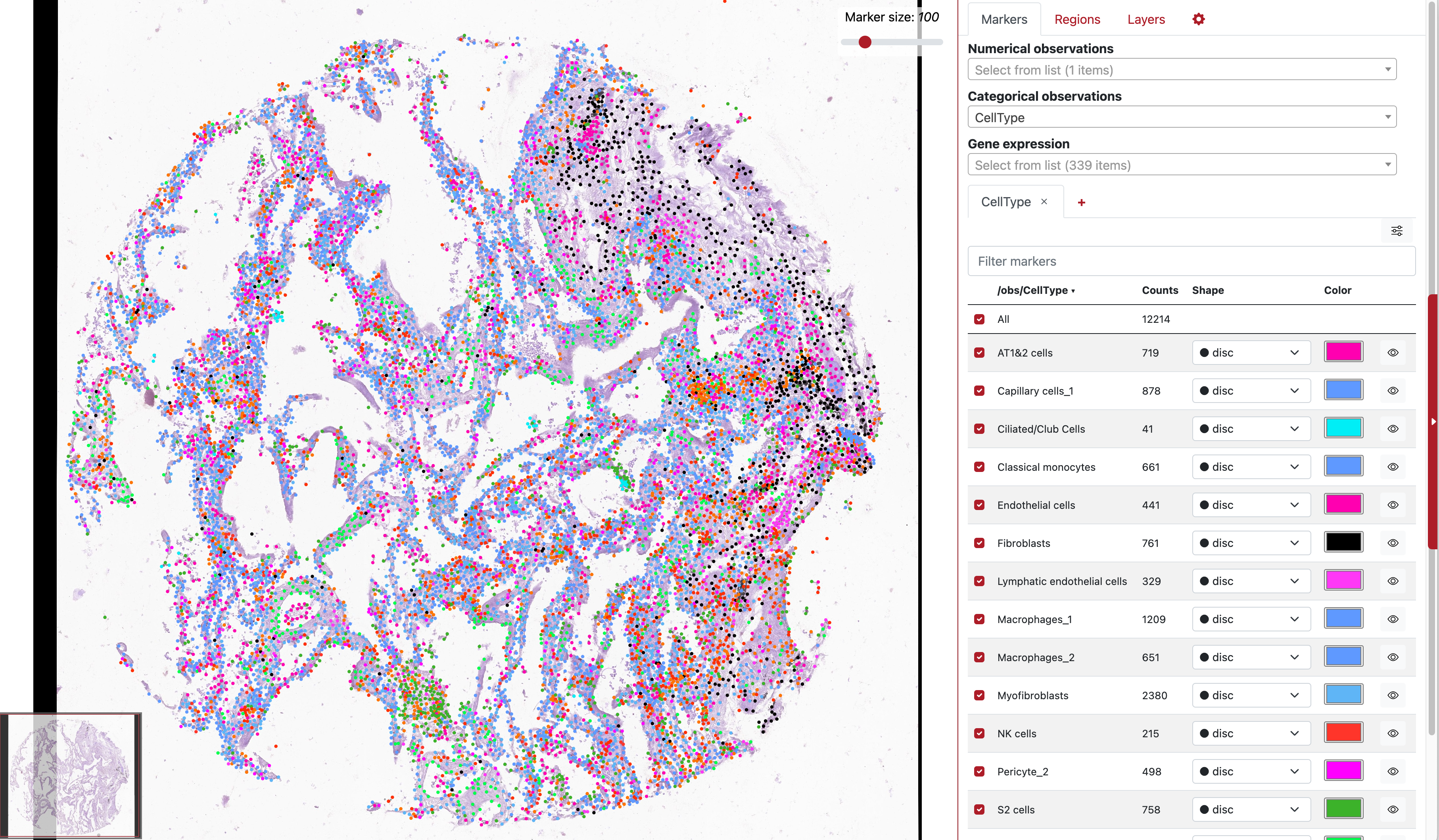
Once the H&E image is registered and transfered to the Xenium data, we can convert the VoltRon object into an Anndata object (h5ad file) and use TissUUmaps tool for interactive visualization.
# convert VoltRon object to h5ad
as.AnnData(vr2_merged_acute1, assay = "Xenium", file = "vr2_merged_acute1.h5ad",
           flip_coordinates = TRUE, name = "main", channel = "H&E")
To run TissUUmaps please follow installation instructions here, then you can simply drag and drop both the h5ad file and png file to the application.
Label Transfer
Now we can transfer ROI annotations as additional metadata features of the molecule assay. We will refer the new metadata column as “Region” which will indicate if the molecule is within any annotated ROI in the same layer.
vrMainAssay(vr2_merged_acute1) <- "ROIAnnotation"
vr2_merged_acute1$Region <- vrSpatialPoints(vr2_merged_acute1)

# set the spatial coordinate system of ROI Annotations assay
vrMainSpatial(vr2_merged_acute1[["Assay9"]]) <- "main_reg"

# transfer ROI annotations to molecules
vr2_merged_acute1 <- transferData(object = vr2_merged_acute1, from = "Assay9", to = "Assay8",
                                  features = "Region")

# Metadata of molecules
Metadata(vr2_merged_acute1, assay = "Xenium_mol")
id assay_id overlaps_nucleus gene qv Assay Layer Sample Region
<char> <char> <int> <char> <num> <char> <char> <char> <char>
1: 281651070371256_cb791e Assay8 0 ENAH 40.00000 Xenium_mol Section1 acute case 1 undefined
2: 281651070371258_cb791e Assay8 1 CD274 40.00000 Xenium_mol Section1 acute case 1 undefined
3: 281651070372515_cb791e Assay8 0 CD163 40.00000 Xenium_mol Section1 acute case 1 undefined
4: 281651070374059_cb791e Assay8 1 CTSL 33.97290 Xenium_mol Section1 acute case 1 undefined
5: 281651070374411_cb791e Assay8 0 C1S 40.00000 Xenium_mol Section1 acute case 1 undefined
---
785787: 281874408669584_cb791e Assay8 0 SFRP2 40.00000 Xenium_mol Section1 acute case 1 undefined
785788: 281874408671410_cb791e Assay8 0 S2_N 40.00000 Xenium_mol Section1 acute case 1 undefined
785789: 281874408672438_cb791e Assay8 0 S100A8 40.00000 Xenium_mol Section1 acute case 1 undefined
785790: 281874408673446_cb791e Assay8 0 TIMP1 29.86642 Xenium_mol Section1 acute case 1 undefined
785791: 281874408673882_cb791e Assay8 0 S2_N 40.00000 Xenium_mol Section1 acute case 1 undefinedThese annotations can be accessed from the default molecule level metadata of the VoltRon object.
vrMainAssay(vr2_merged_acute1) <- "Xenium_mol"
head(table(vr2_merged_acute1$Region))
ROI1_Assay9 ROI10_Assay9 ROI100_Assay9 ROI101_Assay9 ROI102_Assay9 ROI103_Assay9
583 624 784 357 215 200 Now we will grab these annotations from molecule metadata and calculate the ratio of N to orf1ab frequency of SARS‑CoV‑2 particles across all annotated molecules.
library(dplyr)
s2_summary_hyaline <-
  Metadata(vr2_merged_acute1, assay = "Xenium_mol") %>%
  filter(gene %in% c("S2_N", "S2_orf1ab"),
         Region != "undefined") %>%
  summarise(S2_N = sum(gene == "S2_N"),
            S2_orf1ab = sum(gene == "S2_orf1ab"),
            ratio = sum(gene == "S2_N")/sum(gene == "S2_orf1ab")) %>%
  as.matrix()
s2_summary_hyaline
S2_N S2_orf1ab ratio
[1,] 50977 33532 1.520249Manual annotation
To compare the proportion of S2_N and S2_orf1ab molecules in hyaline membranes with tissue sites of possible infection. We focus on another tissue niche where a large accumulation of cells with high S2_N and S2_orf1ab counts.
By visualizing and zooming on a spatial plot with annotated cells, we can detect a site of cells with high infection which are also accompanied by a group of T cells.
vrSpatialPlot(vr2_merged_acute1, assay = "Xenium", group.by = "CellType",
              group.ids = c("H.I. Cells", "T cells"), plot.segments = TRUE,
              alpha = 0.6, spatial = "main", channel = "H&E", interactive = TRUE)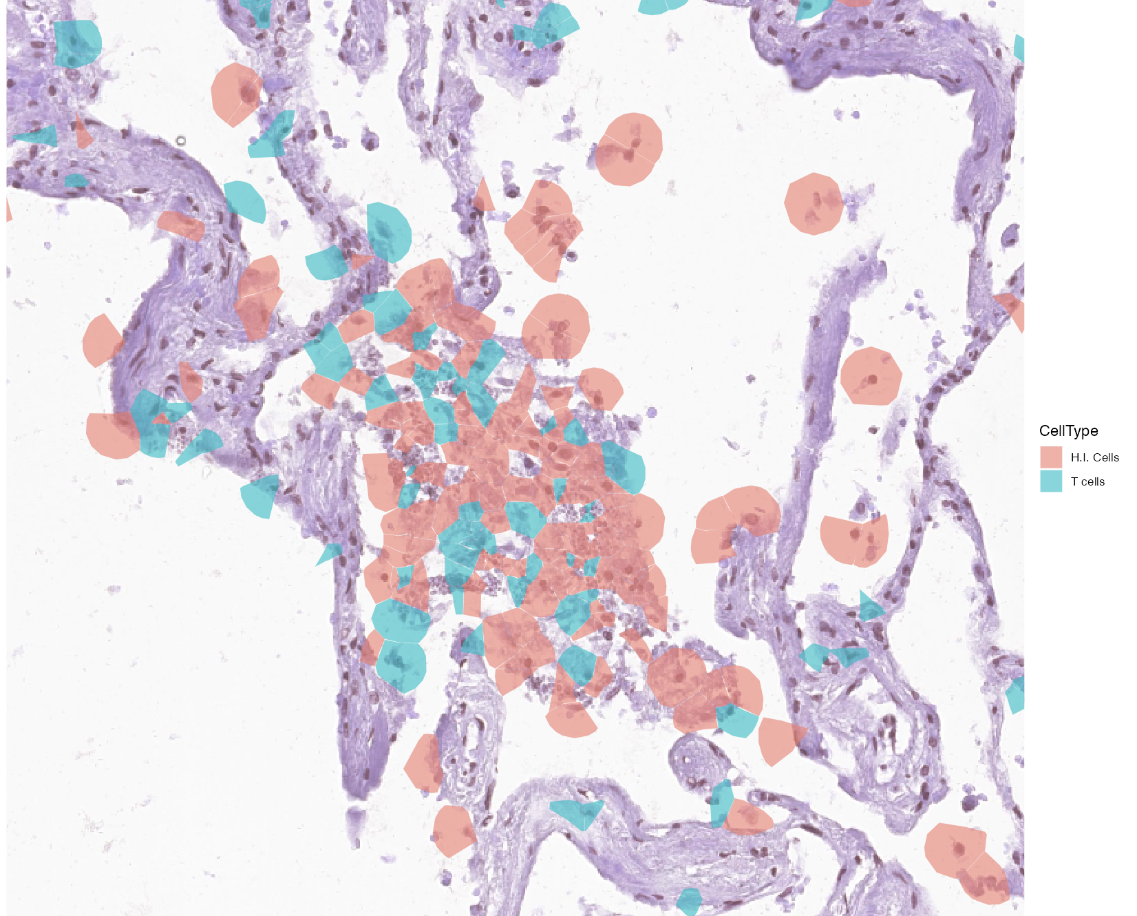
Now we use the annotateSpatialData function to create an additional annotation of Xenium molecules directly. By selecting this region of infection we can directly annotate the ‘Xenium_mol’ assay and the metadata of molecules. We use the H&E image as the background again, and generate a new molecule-level metadata column called “Infected”.
vr2_merged_acute1 <- annotateSpatialData(vr2_merged_acute1, assay = "Xenium_mol",
                                         label = "Region", use.image = TRUE,
                                         channel = "H&E", annotation_assay = "ROIAnnotation1")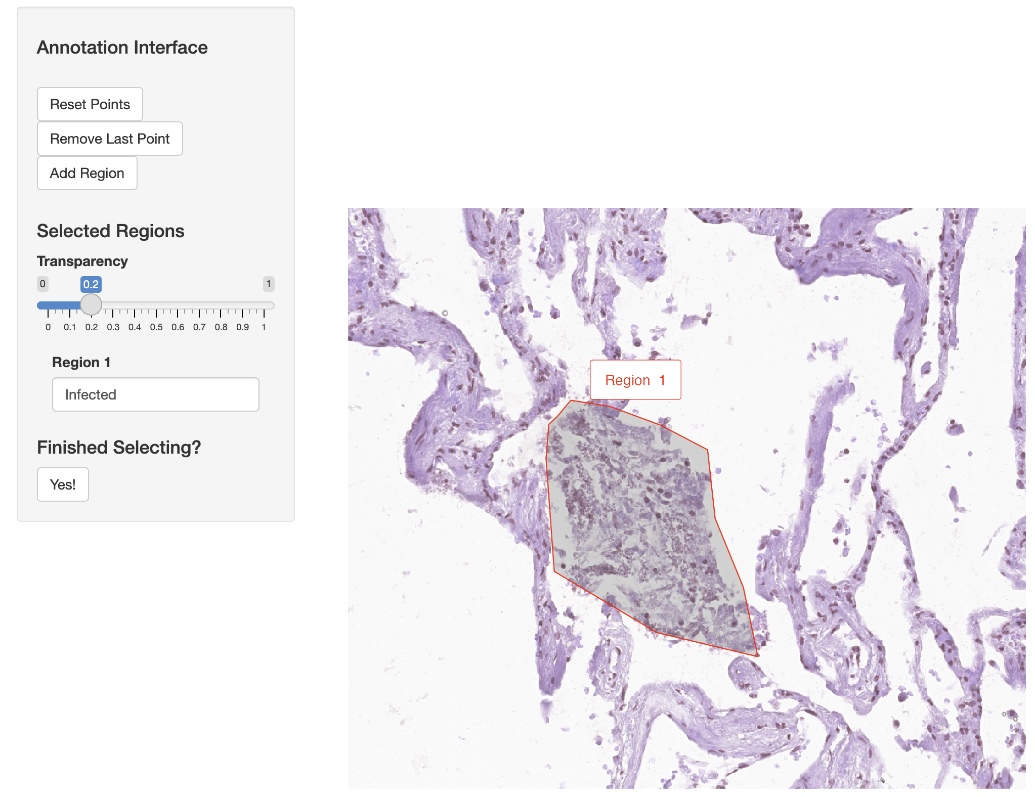
Visualize annotations
Before visualizing the annotations and molecule localizations in the same time, let’s make some changes to the metadata. We basically want to change the annotation of all ROIs originated from the GeoJson file to have the label Hyaline Membrane.
# update molecule metadata
vrMainAssay(vr2_merged_acute1) <- "Xenium_mol"
vr2_merged_acute1$Region <- gsub("ROI[0-9]+", "Hyaline Membrane",
                                 vr2_merged_acute1$Region)

# update ROI metadata
vrMainAssay(vr2_merged_acute1) <- "ROIAnnotation"
vr2_merged_acute1$Region <- gsub("ROI[0-9]+", "Hyaline Membrane",
                                 vr2_merged_acute1$Region)
Now we can visualize two assays together. We use the addSpatialLayer function to overlay molecule locations with both the Hyaline Membrane and the infected region annotations.
vrSpatialPlot(vr2_merged_acute1, assay = "Xenium_mol", group.by = "gene",
              group.ids = c("S2_N", "S2_orf1ab"), n.tile = 500) |>
  addSpatialLayer(vr2_merged_acute1, assay = "ROIAnnotation",
                  group.by = "Region", alpha = 0.3,
                  colors = list(`Hyaline Membrane` = "blue", `Infected` = "yellow"))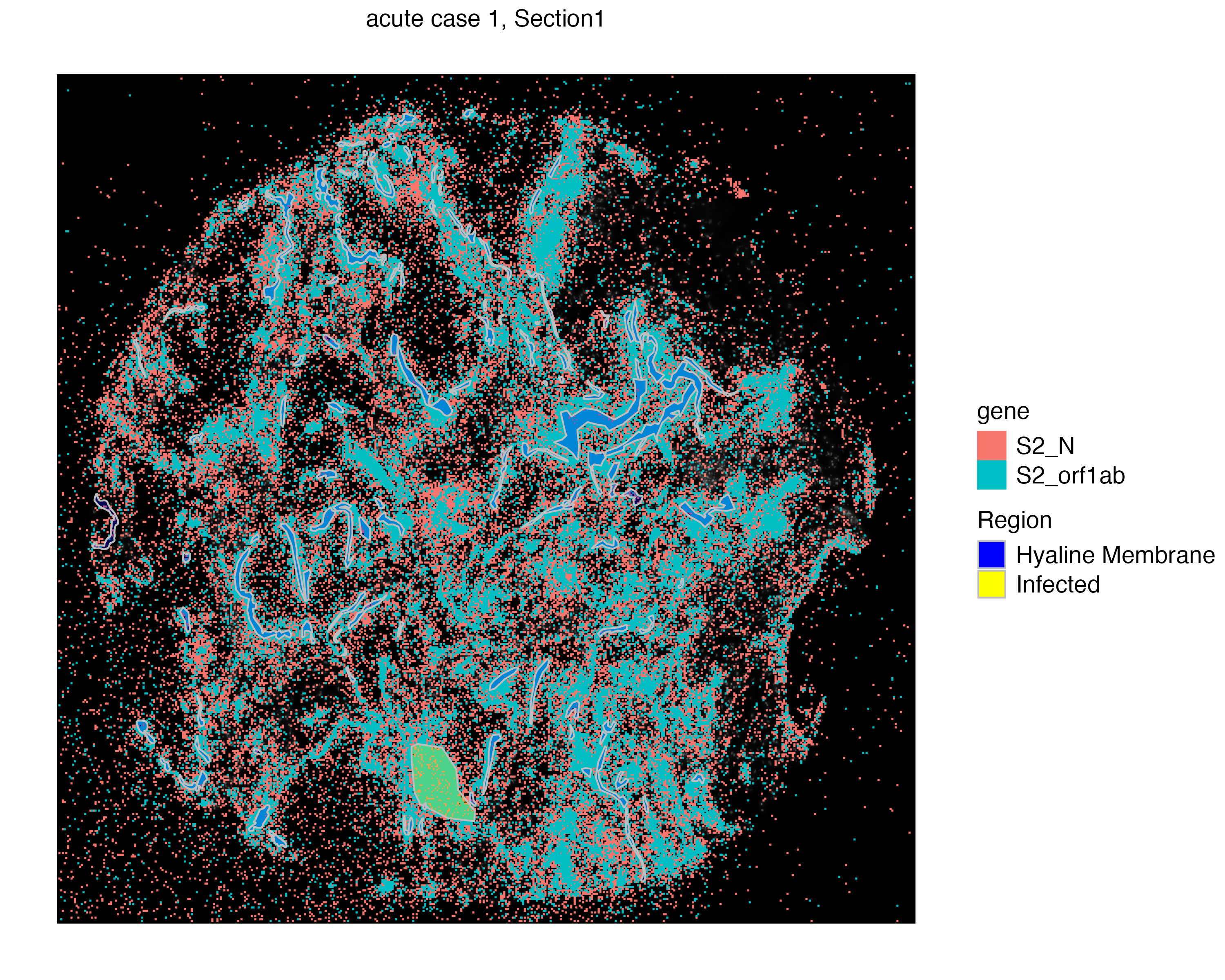
Comparison of annotations
By using the newly annotated infection-associated virus molecules, we can do a comparison of infected regions versus the hyaline membranes.
library(dplyr)
s2_summary_infected <-
  Metadata(vr2_merged_acute1, assay = "Xenium_mol") %>%
  filter(gene %in% c("S2_N", "S2_orf1ab"),
         Region == "Infected") %>%
  summarise(S2_N = sum(gene == "S2_N"),
            S2_orf1ab = sum(gene == "S2_orf1ab"),
            ratio = sum(gene == "S2_N")/sum(gene == "S2_orf1ab")) %>%
  as.matrix()
s2_summary_infected
S2_N S2_orf1ab ratio
[1,] 6376 2372 2.688027Comparison of both the ratio between the infected region and the hyaline membranes show a considerable difference of the population of S2_N and S2_orf1ab molecules.
S2_table <- matrix(c(s2_summary_hyaline[,1:2],
                     s2_summary_infected[,1:2]),
                   dimnames = list(Region = c("Hyaline", "Infected"),
                                   S2 = c("N", "orf1ab")),
                   ncol = 2,  byrow = TRUE)
S2_table
S2
Region N orf1ab
Hyaline 50977 33532
Infected 6376 2372A quick test of independence on this contingency table show a significant difference of ratios across Hyaline and Infected regions.
fisher.test(S2_table, alternative = "two.sided")
    Fisher's Exact Test for Count Data

data:  S2_table
p-value < 2.2e-16
alternative hypothesis: true odds ratio is not equal to 1
95 percent confidence interval:
 0.5382305 0.5941683
sample estimates:
odds ratio
 0.5655696
Xenium Breast Cancer Data
VoltRon allows analyzing biological images, such as H&E stainings of tissue sections, independant to omics assays on either the same or adjacent tissue section. VoltRon defines image tiles, which are collections of image pixels of the same size, and generate latent variables that are analyzed downstream. Unsupervised clustering of these tiles partition regions over the image with respect to morphological features. Here, these regions might be associated to tumor, immune or stroma niches can then be transfered to cells in the same tissue section learn collections of cells with similar features.
We will use the H&E images generated from the same sections as the Xenium In Situ platform, and cluster tiles of the H&E to later transfer groups of tiles to Xenium cells.
You can download the Xenium readout and the H&E image of the same tissue section from the 10x Genomics website (specifically, import In Situ Replicate 1 and Supplemental: Post-Xenium H&E image (TIFF)).
Import Xenium Data
We import both Xenium and post-Xenium H&E images into two separate VoltRon objects and overlay H&E images.
# dependencies
if(!requireNamespace("RBioFormats"))
  BiocManager::install("RBioFormats")
if(!requireNamespace("arrow"))
  install.packages("arrow")
if(!requireNamespace("rhdf5"))
  BiocManager::install("rhdf5")

# import Xenium
Xen_R1 <- importXenium("Xenium_R1/outs",
                       sample_name = "XeniumR1",
                       resolution_level = 3,
                       overwrite_resolution = TRUE)
Xen_R1
Xen_R1_image <- importImageData("Xenium_FFPE_Human_Breast_Cancer_Rep1_he_image.tif",
sample_name = "XeniumR1",
channel_names = "H&E",
tile.size = 128)
Xen_R1_image Clustering
Using VoltRon we can also integrate tile-level spatial entities and image tiles with existing image foundation models such as DinoV2 or UNI. We can parse tiles from VoltRon, and get embedding values from a Foundation model to conduct downstream clustering using PCA and kmeans clustering. See Image tiles/pixels analysis tutorial for more information. You can also download the DinoV2 embeddings from here.
embed_data <- readRDS("img_128_processed.rds")
ind <- sapply(vrSpatialPoints(Xen_R1_image), function(x) strsplit(x, split = "_")[[1]][1])
embed_data <- embed_data[ind,]
rownames(embed_data) <- vrSpatialPoints(Xen_R1_image)
vrEmbeddings(Xen_R1_image, type = "dinov2", overwrite = TRUE) <-  embed_data
Xen_R1_image <- getPCA(Xen_R1_image, dims = 50, data.type = "dinov2")
Xen_R1_image <- getClusters(Xen_R1_image, method = "kmeans", label = "Cluster_kmeans", data.type = "pca", nclus = 10)vrSpatialPlot(Xen_R1_image, group.by = "Cluster_kmeans", alpha = 1)![]()
Automated H&E Registration
In order to transfer the cluster labels of the tiles that partition regions, we need to first syncronize the spatial coordinate systems of the H&E image and the Xenium cells. Here we use the H&E image as the reference image and warp the coordinate system of the Xenium cells using the DAPI channel of the Xenium assay. See Spatial Data Alignment tutorial for more information on image registeration and alignment.
xen_reg <- registerSpatialData(object_list = list(Xen_R1_image, Xen_R1))![]()
We can now parse the registered Xenium data from the result of the registerSpatialData function, and add this assay to the same section as the H&E image.
Xen_R1_reg <- xen_reg$registered_spat[[2]]
Xen_R1_merged <- Xen_R1_image
Xen_R1_merged <- addAssay(Xen_R1_merged,
                          metadata = Metadata(Xen_R1_reg),
                          assay = Xen_R1_reg[["Assay1"]],
                          assay_name = "Xenium",
                          sample = "XeniumR1")
Label Transfer
We can view the combined dataset with the H&E tile data and Xenium assay that are in the same tissue section.
SampleMetadata(Xen_R1_merged) Assay Layer Sample
Assay1 ImageData Section1 XeniumR1
Assay2 Xenium Section1 XeniumR1We would like to transfer the labels of the tiles to cells whose centroids are within a single tile. Thus we transfer Cluster_kmeans from Assay1 (H&E tiles) to Assay2 (Xenium cells). We can also transfer the H&E image to the Xenium assay the second (registered) coordinate system of Xenium data is sync with the H&E image.
# transfer label
Xen_R1_merged <- transferData(Xen_R1_merged,
                              from = "Assay1",
                              to = "Assay2",
                              features = "Cluster_kmeans",
                              expand = FALSE)

# transfer image
vrImages(Xen_R1_merged[["Assay2"]], name = "main_reg", channel = "H&E") <-
  vrImages(Xen_R1_merged, assay = "Assay1")
You can visualize the transferred tile labels in two different spatial coordinate systems and with different images (DAPI, H&E etc.) using spatial and channel arguments, respectively.
vrMainAssay(Xen_R1_merged) <- "Xenium"
vrSpatialPlot(Xen_R1_merged, group.by = "Cluster_kmeans", spatial = "main")
vrSpatialPlot(Xen_R1_merged, group.by = "Cluster_kmeans", spatial = "main_reg",
channel = "H&E")|
|
|
Marker Analysis
Now that we have labelled cells whose partitioning is determined by the morphological (image foundation model) features, we can perform marker analysis to determine signatures associated with groups. We convert the cells assays of the VoltRon object to a Seurat object prior to marker analysis, find markers associated with groups and then parse significant markers to visualize later. See Conversion tutorial for more information on VoltRon’s interoperability features.
library(Seurat)
library(dplyr)
Xen_data_seu <- VoltRon::as.Seurat(Xen_R1_merged, cell.assay = "Xenium", type = "image")
Xen_data_seu <- NormalizeData(Xen_data_seu, scale.factor = 100)
Idents(Xen_data_seu) <- "Cluster_kmeans"
markers_image <- FindAllMarkers(Xen_data_seu)
markers_image_top <- markers_image %>%
  group_by(cluster) %>%
  dplyr::filter(avg_log2FC > 1, p_val_adj < 0.05, pct.1 > 0.5)
head(as.data.frame(markers_image_top))
p_val avg_log2FC pct.1 pct.2 p_val_adj cluster gene
1 0 1.679807 0.787 0.335 0 8 MLPH
2 0 1.406676 0.869 0.430 0 8 KRT8
3 0 1.442903 0.782 0.359 0 8 CDH1
4 0 1.693801 0.808 0.385 0 8 FASN
5 0 1.526783 0.874 0.458 0 8 EPCAM
6 0 1.493334 0.670 0.259 0 8 MYO5BHeatmap visualization of these clusters reveal markers of tumor, stroma and immune niches.
Xen_R1_merged <- normalizeData(Xen_R1_merged, sizefactor = 1000)
vrHeatmapPlot(Xen_R1_merged, group.by = "Cluster_kmeans",
              features = unique(markers_image_top$gene),
show_row_names = TRUE)![]()
Inspecting the heatmap and the spatial plot simultanuously, we can see that some tiles are associated with the H&E background where others are representing tumor, immune and stroma niches.
annotation <- Xen_R1_merged$Cluster_kmeans
annotation[annotation %in% c(6,8)] <- "Tumor Niche"
annotation[annotation %in% c(1)] <- "Immune Niche"
annotation[annotation %in% c(2,10,9)] <- "Stroma"
annotation[annotation %in% c(4)] <- "Stroma"
annotation[annotation %in% c(3,5,7)] <- "Background"
Xen_R1_merged$annotation <- annotation
Users can also visualize tile and cell simultaneously and their features.
# select a subset
Xen_R1_image_subset <- subset(Xen_R1_merged, interactive = TRUE)
Xen_R1_image_subset <- Xen_R1_image_subset$subsets[[1]]

# visualize
vrSpatialPlot(Xen_R1_image_subset, group.by = "Cluster_kmeans", alpha = 0.7)
vrSpatialPlot(Xen_R1_image_subset, assay = "Xenium", group.by = "annotation",
alpha = 0.7, plot.segments = TRUE, channel = "H&E")![]()
vrSpatialFeaturePlot(Xen_R1_image_subset, assay = "Xenium",
                     features = c("PTPRC", "EPCAM", "MMP2"),
alpha = 0.7, plot.segments = TRUE, ncol = 2)![]()
Xenium + IF Tonsil Data
Automated alignment workflow of VoltRon can also be used to integrate modalities generated from the same tissue section. In this use case, we will perform multiplex immunofluorescence (IF) imaging after a Xenium experiment and integrate Protein and RNA modalities for clustering.
Import Xenium Data
We will generate Xenium and IF dataset from a human tonsil tissue section. We first import the Xenium data, and interactively subset the tonsil sample from the tissue microarray.
You can also download the tonsil subset from here.
# dependencies
if(!requireNamespace("RBioFormats"))
  BiocManager::install("RBioFormats")
if(!requireNamespace("arrow"))
  install.packages("arrow")
if(!requireNamespace("rhdf5"))
  BiocManager::install("rhdf5")

# import Xenium
xen <- importXenium("Xenium/outs",
                    sample_name = "XeniumTonsil",
                    resolution_level = 3,
                    overwrite_resolution = TRUE)

# subset interactive
xen <- subset(xen, interactive = TRUE)
xen_tonsil <- xen$subsets[[1]]

# load from RDS if needed
# xen_tonsil <- readRDS("Xenium_tonsil_subset.rds")

# view image
vrImages(xen_tonsil)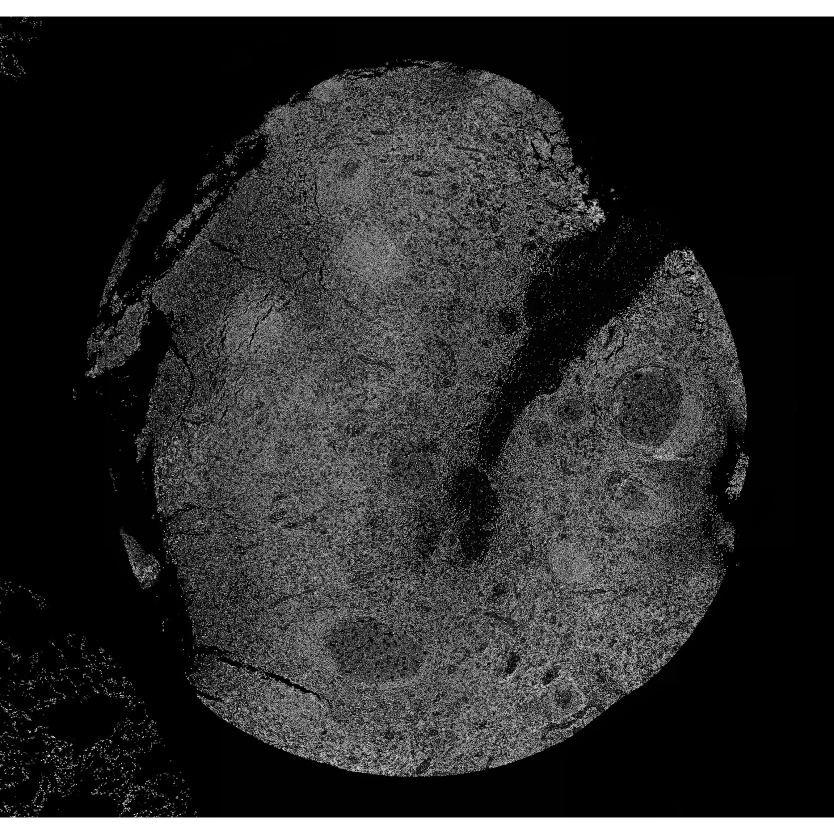
Import IF Images
Xenium in situ platform allows same section multiplex imaging post experiment. Depending on the protocol, the intensity measures of each channel can be stored in an ome.tiff file. We use the importImageData to import the images of channels where we can select channels and even give them names.
We import only the DAPI, CD20 and CD21 channels. We will use DAPI channel for aligning these images to Xenium data, and remaining channels for clustering with the RNA features from Xenium.
You can download the ome.tiff file of the same section IF experiment here.
if_tonsil <- importImageData("same_section_IF.ome.tif", tile.size = 100,
                             series = 1, resolution = 1, channels = c(1,4,8),
                             channel_names = c("DAPI", "CD20", "CD21"),
                             is.RGB = FALSE)
Automated Alignment
Now, we perform automated alignment across Xenium and IF datasets.
xen_tonsil <- modulateImage(xen_tonsil, brightness = 500)
if_tonsil <- modulateImage(if_tonsil, brightness = 700, channel = "DAPI")
xen_reg <- registerSpatialData(object_list = list(if_tonsil, xen_tonsil))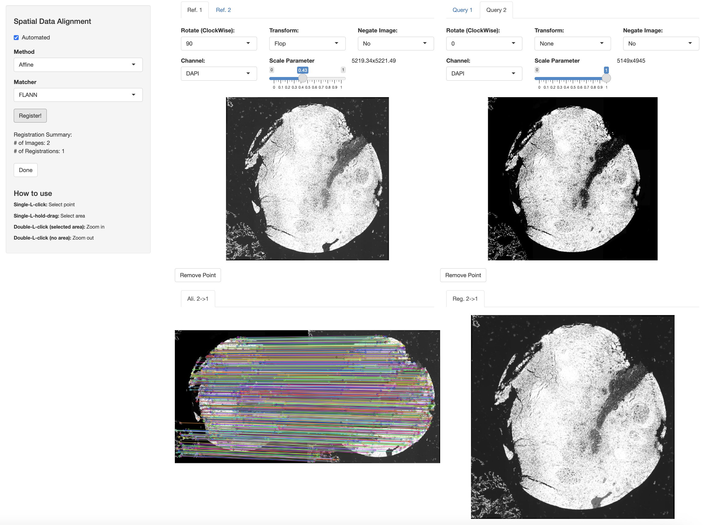
The output of the registerSpatialData function will include a VoltRon object of the Xenium data whose cell segments are syncronized to the IF experiment.
# get registered data
xen_tonsil <- xen_reg$registered_spat[[2]]
We can also transfer the CD20, and CD21 channels to the registered coordinate space of the Xenium data.
vrImages(xen_tonsil[["Assay1"]], name = "main_reg", channel = "CD20") <-
  vrImages(if_tonsil, channel = "CD20")
vrImages(xen_tonsil[["Assay1"]], name = "main_reg", channel = "CD21") <-
  vrImages(if_tonsil, channel = "CD21")
Quantify Intensity of Cells
With VoltRon, we can export the registered segments, and save it as a GeoJson file for further processing with QuPath, which we will use it to quantify the mean intensity measures of CD20 and CD21 protein per Xenium segments.
This will enable collecting same segment RNA and Protein measures for multi-modal clustering.
segts <- vrSegments(flipCoordinates(xen_tonsil))
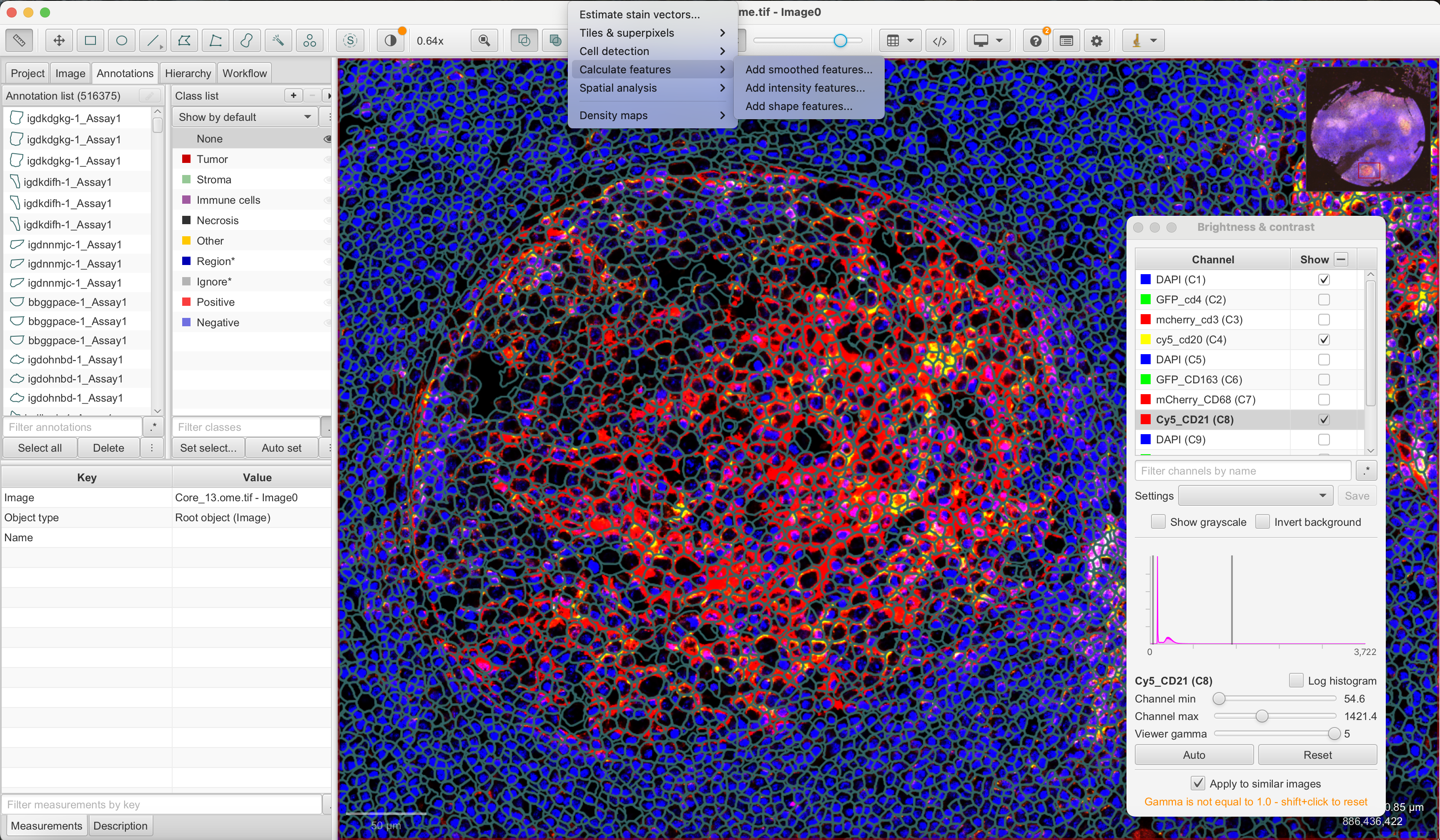
generateGeoJSON(segts, "registered_segments.geojson")To perform intensity quantification of cells, simply drag and drop the ome.tiff and geojson files to QuPath. You can then navigate to Analyze -> Calculate Features -> Add Intensity Features, and click Run after selecting markers where we select CD20 and CD21. If you want to perform the mean and median intensity calculation of features, you can use the GeoJSON file with registered segments found here.
After calculating mean and median intensities, we navigate to Measure -> Show Annotation Measurements and click Save to write the measurements to a .txt file.
After quantifying with QuPath, we can import these measures and save it as a new feature data in VoltRon object. You can find the IF measurements of CD20 and CD21 markers here.
# add feature from QuPath
datax <- read.table("IF_measurements.txt",
                    header = TRUE, sep = "\t")
rownames(datax) <- datax$Name
datax <- datax[vrSpatialPoints(xen_tonsil),]
datax <- datax[,c(11,13)]
datax <- apply(datax, 2, function(x){
  x[is.na(x)] <- min(x, na.rm = TRUE)
  x
})

# adjust channel intensities
datax[,1] <- ifelse(datax[,1] < 1054, datax[,1],1054)
datax[,1] <- ifelse(datax[,1] > 331, datax[,1],331)
datax[,1] <- datax[,1] - min(datax[,1])
datax[,2] <- ifelse(datax[,2] < 1421, datax[,2],1421)
datax[,2] <- ifelse(datax[,2] > 491, datax[,2],491)
datax[,2] <- datax[,2] - min(datax[,2])
colnames(datax) <- c("CD20", "CD21")
We use the addFeature function to import the new Protein measures as additional feature sets
# add as protein features
xen_tonsil <- addFeature(xen_tonsil, data = t(datax), feature_name = "Protein")
xen_tonsil
VoltRon Object
XeniumTonsil:
Layers: Section1
Assays: Xenium(Main)
Features: RNA(Main) Protein Processing Modalities
We first do a simple filtering on the Xenium cells, remove all cells whose total mRNA counts are lower than 30, and we normalize these counts afterwards.
# subset
spatialpoints <- vrSpatialPoints(xen_tonsil)[as.vector(Metadata(xen_tonsil)$Count > 30)]
xen_tonsil <- subset(xen_tonsil, spatialpoints = spatialpoints)

# normalize RNA
xen_tonsil <- normalizeData(xen_tonsil, sizefactor = 1000)
VoltRon also includes methods to process protein intensity measures. We use the hyperbolic arcsine transformation with scaling parameter 0.2.
# normalize Protein markers
vrMainFeatureType(xen_tonsil) <- "Protein"
xen_tonsil <- normalizeData(xen_tonsil, method = "hyper.arcsine", scale = 0.2)
We can visualize spatial localization of both normalized Protein and RNA features. CD20 and MS4A1 are Protein and RNA synonyms of the same marker, hence they largely co-localize. On the other hand, CD38 and CD21 are both markers of germinal centers of human tonsils, but CD21 mainly expressed in these centers and CD38 can also be expressed in plasma cells
library(patchwork)
vrMainFeatureType(xen_tonsil) <- "Protein"
g1 <- vrSpatialFeaturePlot(xen_tonsil, features = c("CD20", "CD21"),
                           background.color = "black", n.tile = 300, ncol = 2,
                           norm = TRUE)
vrMainFeatureType(xen_tonsil) <- "RNA"
g2 <- vrSpatialFeaturePlot(xen_tonsil, features = c("MS4A1", "CD38"),
                           background.color = "black", n.tile = 300, ncol = 2)
g1 / g2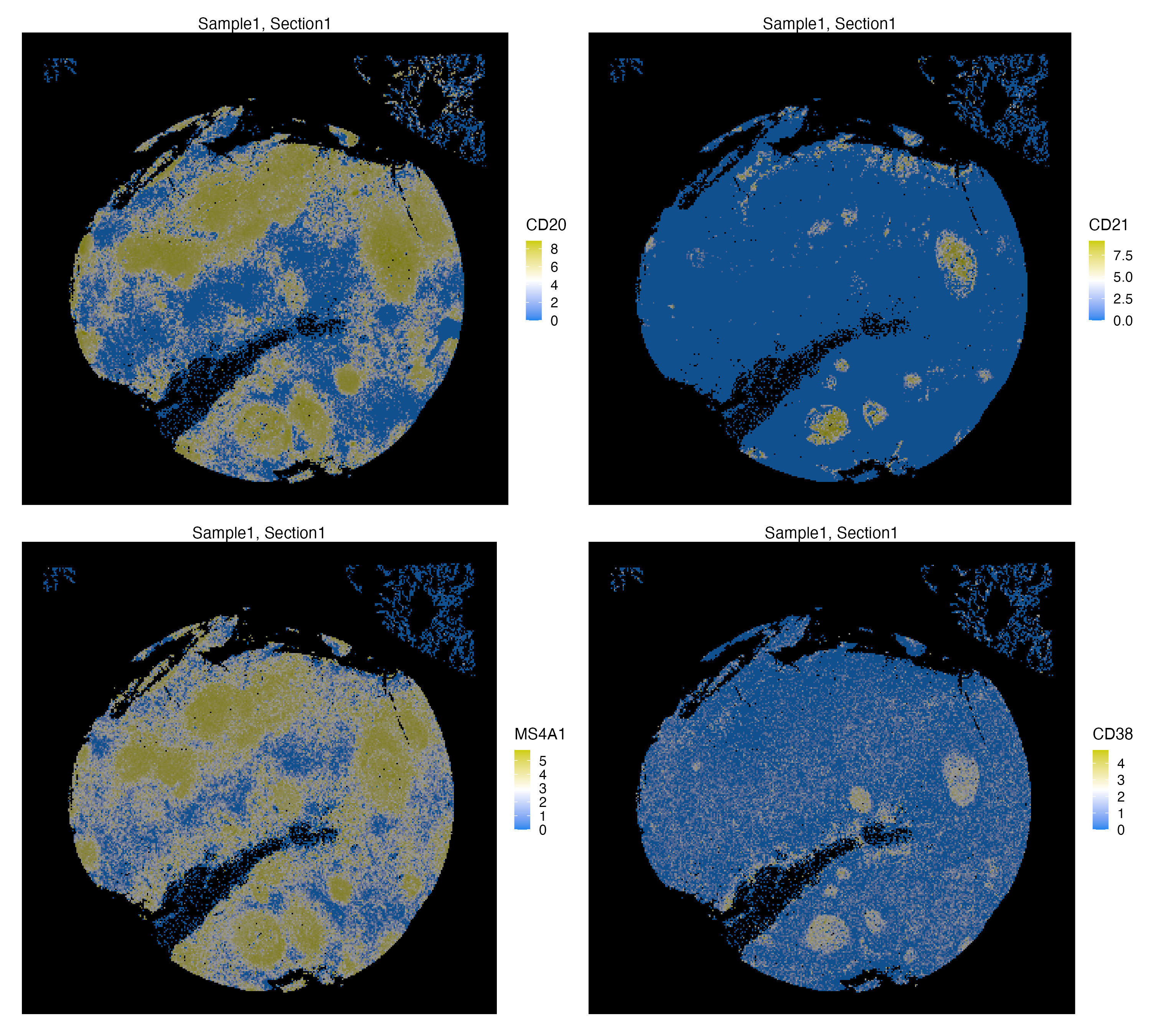
OnDisk (Optional)
VoltRon provides additional utilities to save object on disk to lower memory usage of data analysis and clustering. We can save the object on disk and continue analysis which will potentially increase the clustering speed.
xen_tonsil <- saveVoltRon(xen_tonsil,
                               format = "HDF5VoltRon",
                               output = "data/OnDisk/Xenium_IF",
                               replace = TRUE)
Clustering
We can now apply dimensional reduction which will allow us to cluster cells. The feat_type argument in the getPCA function will accept multiple modality names of a VoltRon object. Here, vrFeatureTypeNames will provide the names of all modalities and will result in getPCA computing PC dimensions using both RNA and Protein modalities.
xen_tonsil <- getPCA(xen_tonsil,
                     feat_type = vrFeatureTypeNames(xen_tonsil),
                     dims = 30)
xen_tonsil <- getUMAP(xen_tonsil, dims = 1:30)
Let us visualize the expression of RNA and Protein features. We can see that CD21 (Protein) and CD38 (RNA) features, which both are germinal center markers, are expressed in different combinations. Also, CD20 and its RNA counterpart MS4A1 show similar expression patterns.
# visualize embeddings
vrMainFeatureType(xen_tonsil) <- "Protein"
g1 <- vrEmbeddingFeaturePlot(xen_tonsil,
                       features = c("CD20", "CD21"), embedding = "umap",
                       pt.size = 0.4)
vrMainFeatureType(xen_tonsil) <- "RNA"
g2 <- vrEmbeddingFeaturePlot(xen_tonsil,
                       features = c("MS4A1", "CXCL13"), embedding = "umap",
                       pt.size = 0.4)
g1 / g2
Clustering with multi-modal PCA will reveal clusters high in both RNA and Protein features. We first cluster the cells using SNN based graph clustering, and then visualize the expression of CD21 to detect marker specific clusters.
# clustering
xen_tonsil <- getProfileNeighbors(xen_tonsil,
                                  dims = 1:30, method = "SNN")
xen_tonsil <- getClusters(xen_tonsil, resolution = 1.0,
                          label = "Clusters", graph = "SNN")

# visualize
vrEmbeddingPlot(xen_tonsil, group.by = "Clusters", embedding = "umap",
                pt.size = 0.4, label = TRUE)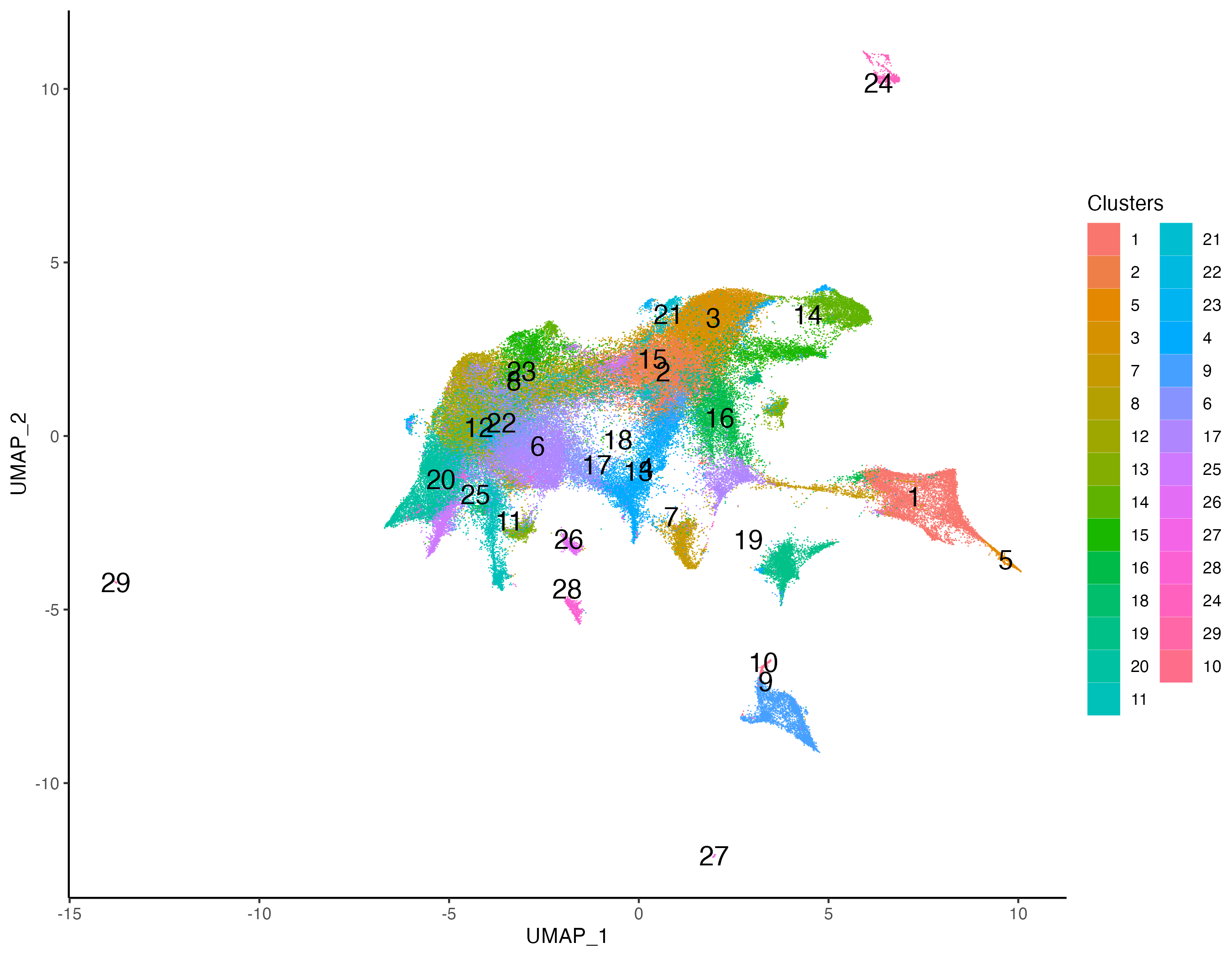
As observed, there is one cluster with high CD21 protein expression.
vrViolinPlot(xen_tonsil, features = "CD21", group.by = "Clusters")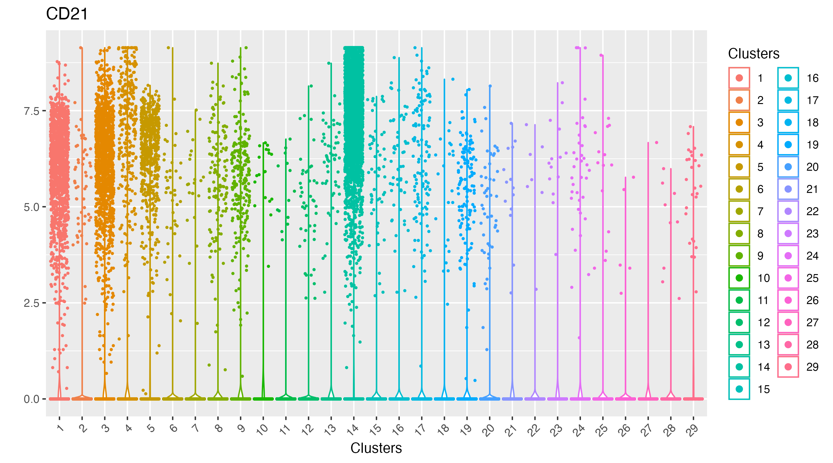
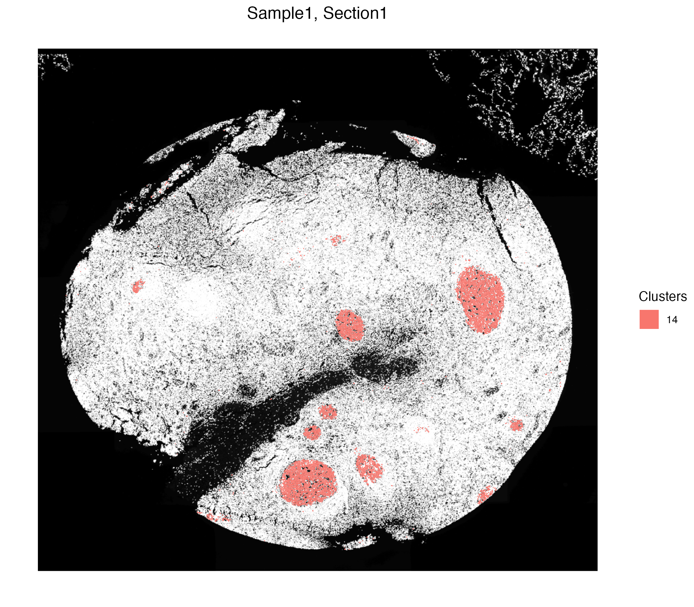
We can visualize the spatial localization of this cluster alone, which point to the germinal centers of the human tonsil.
vrSpatialPlot(xen_tonsil, group.by = "Clusters", group.ids = 14,
              plot.segments = TRUE)