Niche Clustering

Spot-based Niche Clustering

Spot-based spatial transcriptomic assays capture spatially-resolved gene expression profiles that are somewhat closer to single cell resolution. However, each spot still include a few number of cells that are likely from a combination of cell types within the tissue of origin. RNA deconvolution is then incorporated to estimate the percentage/abundance of these cell types within each spot/ROI given a reference scRNAseq dataset.

VoltRon includes wrapper commands for using popular RNA deconvolution methods such as RCTD (spot) and return estimated abundances as additional assays within each layer. These estimated percentages of cell types each spot could be incorporated to detect niches (i.e. small local microenvironments of cells) within the tissue. We can process cell type abundance assays and used them for clustering to detect these niches.

Import Visium Data

For this tutorial we will analyze spot-based transcriptomic assays from Mouse Brain generated by the Visium instrument. The Mouse Brain Serial Section 1/2 datasets can be downloaded from here (specifically, please filter for Species=Mouse, AnatomicalEntity=brain, Chemistry=v1 and PipelineVersion=v1.1.0).

We will now import each of four samples separately and merge them into one VoltRon object. There are four sections in total given two serial anterior and serial posterior sections, hence we have two tissue blocks each having two layers.

library(VoltRon)
Ant_Sec1 <- importVisium("Sagittal_Anterior/Section1/", sample_name = "Anterior1")
Ant_Sec2 <- importVisium("Sagittal_Anterior/Section2/", sample_name = "Anterior2")
Pos_Sec1 <- importVisium("Sagittal_Posterior/Section1/", sample_name = "Posterior1")
Pos_Sec2 <- importVisium("Sagittal_Posterior/Section2/", sample_name = "Posterior2")

# merge datasets
MBrain_Sec_list <- list(Ant_Sec1, Ant_Sec2, Pos_Sec1, Pos_Sec2)
MBrain_Sec <- merge(MBrain_Sec_list[[1]], MBrain_Sec_list[-1], 
                    samples = c("Anterior", "Anterior", "Posterior", "Posterior"))
MBrain_Sec

VoltRon Object 
Anterior: 
  Layers: Section1 Section2 
Posterior: 
  Layers: Section1 Section2 
Assays: Visium(Main) 
Features: RNA(Main) 

VoltRon maps metadata features on the spatial images, multiple features can be provided for all assays/layers associated with the main assay (Visium).

vrSpatialFeaturePlot(MBrain_Sec, features = "Count", crop = TRUE, alpha = 1, ncol = 2)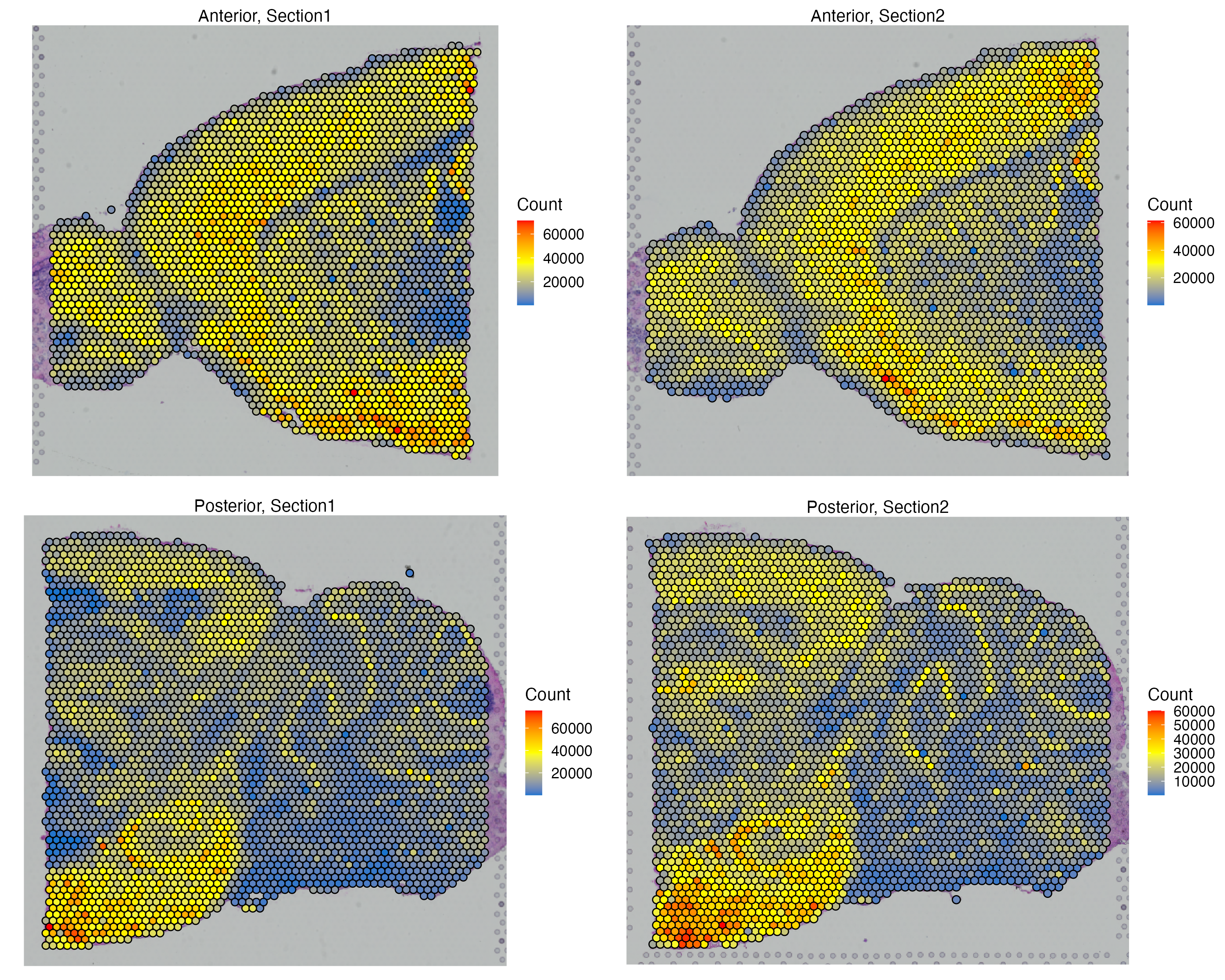

Import scRNA data

We will now import the scRNA data for reference which can be downloaded from here. Specifically, we will use a scRNA reference of Mouse cortical adult brain with 14,000 cells from the Allen Institute, generated with the SMART-Seq2 protocol. This scRNA data is also used by the Spatial Data Analysis tutorial in Seurat website.

Before deconvoluting Visium spots, we correct cell types labels and drop some cell types with extremely few number of cells (e.g. “CR”).

library(Seurat)
allen_reference <- readRDS("allen_cortex.rds")

# process and reduce dimensionality
library(dplyr)
allen_reference <- SCTransform(allen_reference, ncells = 3000, verbose = FALSE) %>%
  RunPCA(verbose = FALSE) %>%
  RunUMAP(dims = 1:30)

# update labels and subset
allen_reference$subclass <- gsub("L2/3 IT", "L23 IT", allen_reference$subclass)
allen_reference <- allen_reference[,colnames(allen_reference)[!allen_reference@meta.data$subclass %in% "CR"]]

# visualize
Idents(allen_reference) <- "subclass"
gsubclass <- DimPlot(allen_reference, reduction = "umap", label = T) + NoLegend()
Idents(allen_reference) <- "class"
gclass <- DimPlot(allen_reference, reduction = "umap", label = T) + NoLegend()
gsubclass | gclass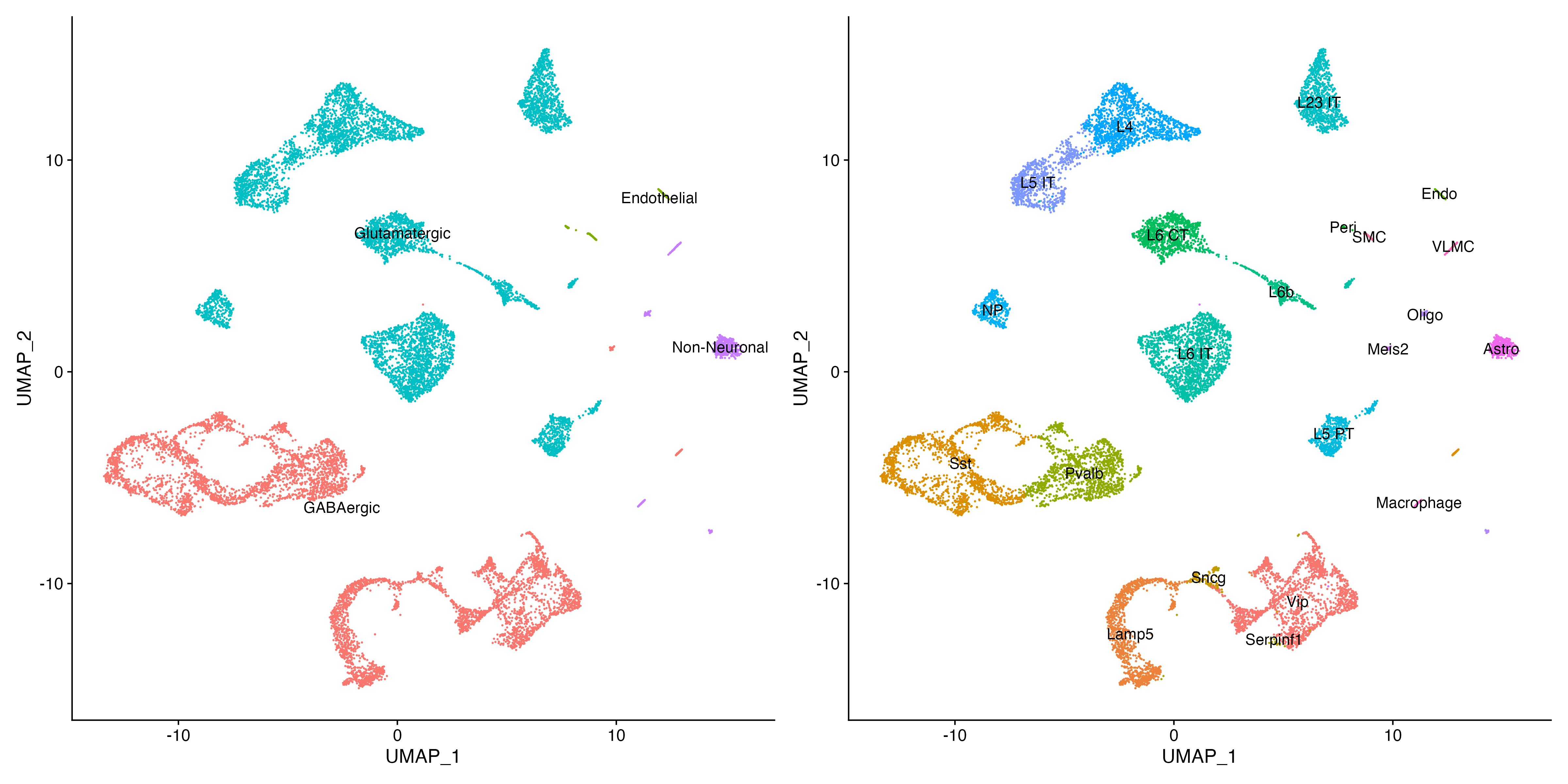

Spot Deconvolution with RCTD

In order to integrate the scRNA data and the Visium data sets within the VoltRon objects, we will use RCTD algorithm which is accessible with the spacexr package.

if(requireNamespace("spacexr"))
  devtools::install_github("dmcable/spacexr", build_vignettes = FALSE)

After running getDeconvolution, an additional assay within the same layer with **_decon** postfix will be created for all layers with a Visium data.

library(spacexr)
MBrain_Sec <- getDeconvolution(MBrain_Sec, sc.object = allen_reference, sc.cluster = "subclass", max_cores = 6)
MBrain_Sec

VoltRon Object 
Anterior: 
  Layers: Section1 Section2 
Posterior: 
  Layers: Section1 Section2 
Assays: Visium(Main) 
Features: RNA(Main) Decon 

We can now switch to the Decon feature type where features are cell types from the scRNA reference and the data values are cell types percentages in each spot.

vrMainFeatureType(MBrain_Sec) <- "Decon"
vrFeatures(MBrain_Sec)

 [1] "Astro"      "Endo"       "L23 IT"     "L4"         "L5 IT"      "L5 PT"     
 [7] "L6 CT"      "L6 IT"      "L6b"        "Lamp5"      "Macrophage" "Meis2"     
[13] "NP"         "Oligo"      "Peri"       "Pvalb"      "Serpinf1"   "SMC"       
[19] "Sncg"       "Sst"        "Vip"        "VLMC"          

These features (i.e. cell type abundances) can be visualized like all other feature types.

vrSpatialFeaturePlot(MBrain_Sec, features = c("L4", "L5 PT", "Oligo", "Vip"), 
                     crop = TRUE, ncol = 2, alpha = 1, keep.scale = "all")

Clustering

Relative cell type abundances that are learned by RCTD and stored within VoltRon can now be used to cluster spots. These groups or clusters of spots can also be realized as niches, regions within tissue sections that have a distinct cell type composition compared to the remaining parts of the tissue.

We will now normalize and process relative cell type abundances to learn/detect these niche clusters. We treat cell type abundances as compositional data, hence we incorporate centred log ratio (CLR) transformation for normalizing them.

MBrain_Sec <- normalizeData(MBrain_Sec, method = "CLR")

The CLR normalized assay have only 25 features, each representing a cell type from the single cell reference data. Hence, we can directly calculate UMAP reductions from this feature set without relying on a prior dimensionality reduction such as PCA.

VoltRon is also capable of calculating the UMAP reduction from normalized data slots. Hence, we build a UMAP reduction from CLR data. However, UMAP will always be calculated from a PCA reduction by default (if a PCA embedding is found in the object).

MBrain_Sec <- getUMAP(MBrain_Sec, data.type = "norm")
vrEmbeddingPlot(MBrain_Sec, embedding = "umap", group.by = "Sample")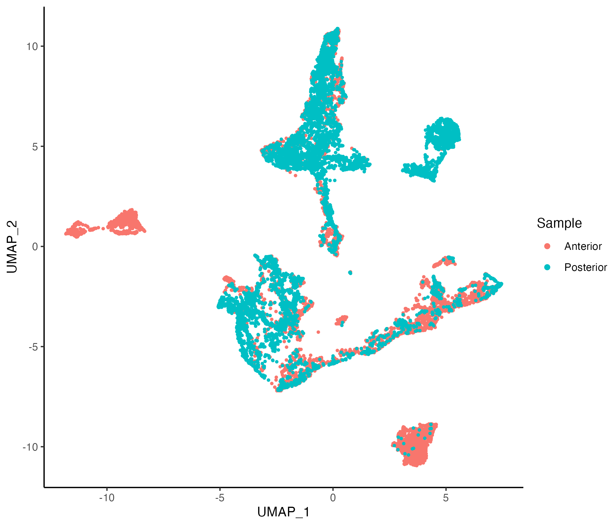

Using normalized cell type abundances, we can now generate k-nearest neighbor graphs and cluster the graph using leiden method.

MBrain_Sec <- getProfileNeighbors(MBrain_Sec, data.type = "norm", method = "SNN")
MBrain_Sec <- getClusters(MBrain_Sec, resolution = 0.6, graph = "SNN")

Visualization

VoltRon incorporates distinct plotting functions for, e.g. embeddings, coordinates, heatmap and even barplots. We can now map the clusters we have generated on UMAP embeddings.

# visualize 
g1 <- vrEmbeddingPlot(MBrain_Sec, embedding = "umap", group.by = "Sample")
g2 <- vrEmbeddingPlot(MBrain_Sec, embedding = "umap", group.by = "clusters", label = TRUE)
g1 | g2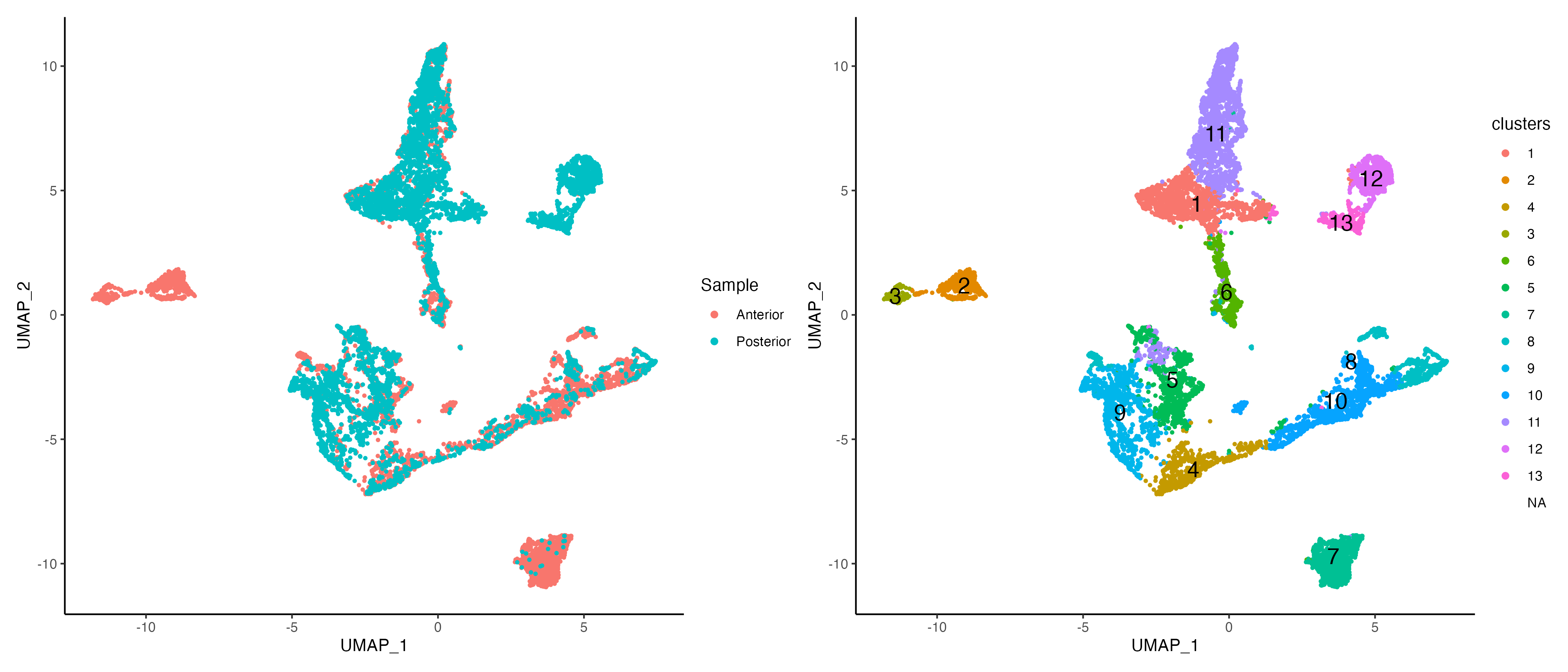

Mapping clusters on the spatial images and spots would show the niche structure across the tissues and layers.

vrSpatialPlot(MBrain_Sec, group.by = "clusters", crop = TRUE, alpha = 1)

We use vrHeatmapPlot to investigate relative cell type abundances across these niche clusters. You will need to have ComplexHeatmap package in your namespace.

library(ComplexHeatmap)
vrHeatmapPlot(MBrain_Sec, features = vrFeatures(MBrain_Sec), group.by = "clusters", 
              show_row_names = T, show_heatmap_legend = T)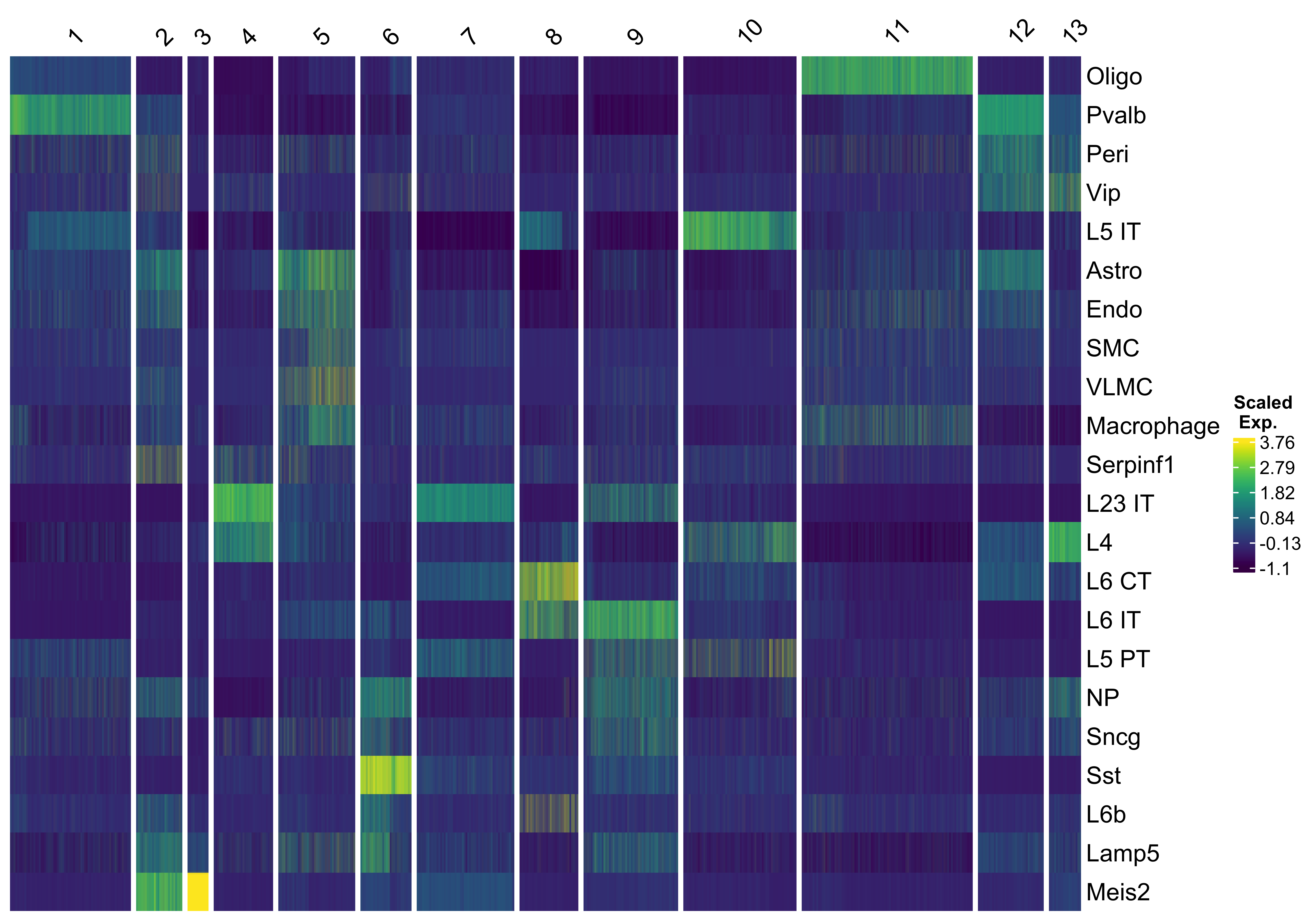

Cell-based Niche Clustering

Unlike spot-based assays, spatial transcriptomics data in single cell resolution require building niche assays to detect clusters that are equivalent to the niches that each individual cell belongs to. We first detect the mixture of cells around a spatial neighborhood around each of these cells and use that a profile to perform clustering.

Import Xenium Data

For this, the data has to be already clustered (and annotated if possible). We will use the cluster labels generated at the end of the Xenium analysis section of workflow from Cell/Spot Analysis. You can download the VoltRon object with clustered and annotated Xenium cells along with the Visium assay from here.

Xen_data <- readRDS("VRBlock_data_clustered.rds")
vrMainSpatial(Xen_data, assay = "Assay1") <- "main"
vrMainSpatial(Xen_data, assay = "Assay3") <- "main"
vrSpatialPlot(Xen_data, group.by = "CellType", pt.size = 0.13, background = "black", 
              legend.loc = "top", n.tile = 500)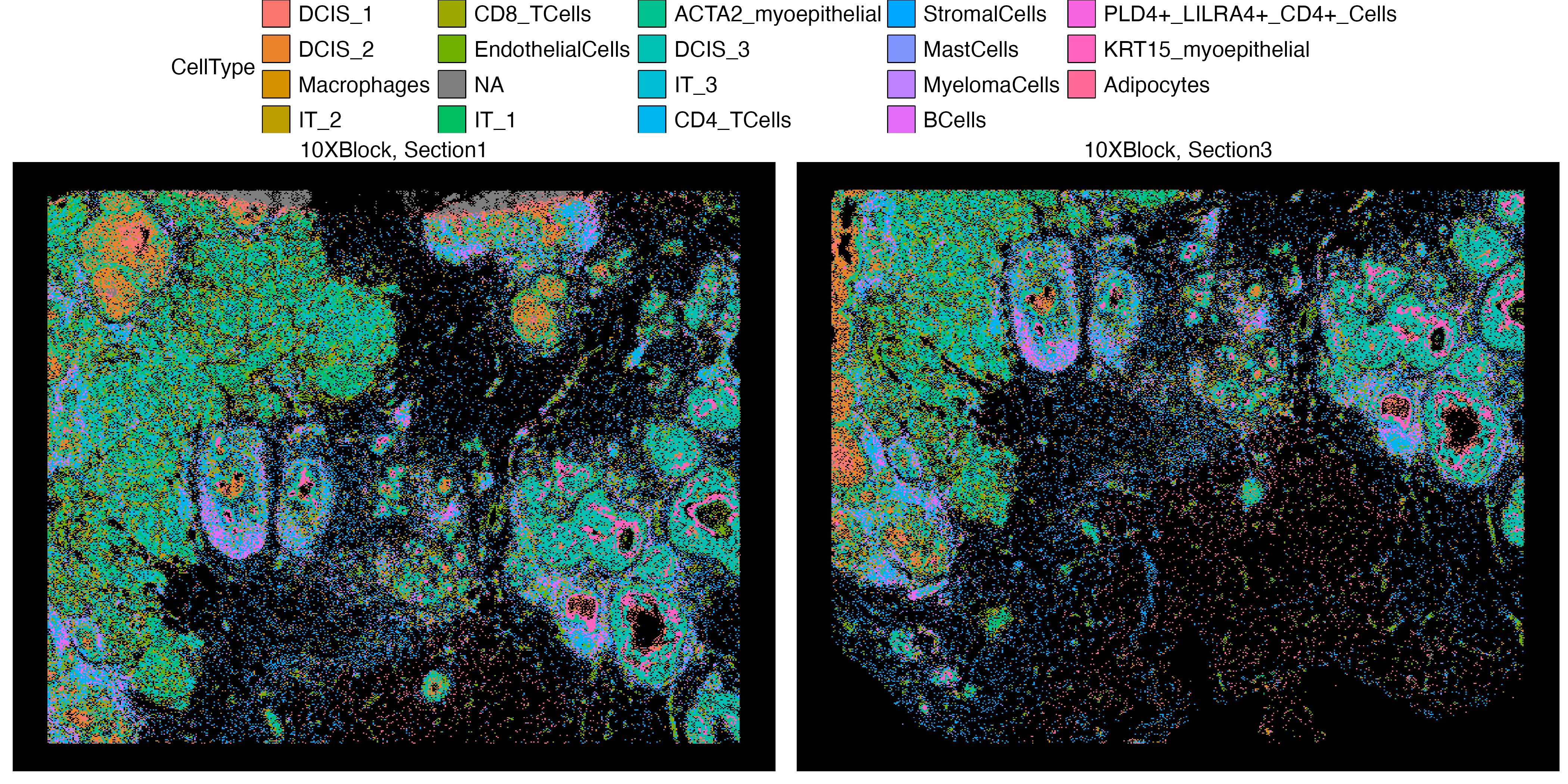

Creating Niche Assay

Here, in order to calculate niche profiles for each cell, we have to first build spatial neighborhoods around cells and capture the local cell type mixtures. Using getSpatialNeighbors, we build a spatial neighborhood graph to connect all cells to other cells within at most 15 distance apart

Xen_data <- getSpatialNeighbors(Xen_data, radius = 15, method = "radius")
vrGraphNames(Xen_data)

[1] "radius"

Now, we can build a niche assay for cells using the getNicheAssay function which will create an additional feature set for cells called Niche. Here, each cell type is a feature and the profile of a cell represents the relative abundance of cell types around each cell.

Xen_data <- getNicheAssay(Xen_data, label = "CellType", graph.type = "radius")
Xen_data

VoltRon Object 
10XBlock: 
  Layers: Section1 Section2 Section3 
Assays: Xenium(Main) Visium 
Features: RNA(Main) Niche

Clustering

The Niche assay can be normalized similar to the spot-level niche analysis using centred log ratio (CLR) transformation.

vrMainFeatureType(Xen_data) <- "Niche"
Xen_data <- normalizeData(Xen_data, method = "CLR")

Default clustering functions could be used to analyze the normalized niche profiles of cells to detect niches associated with each cell. However, we use K-means algorithm to perform the niche clustering.

Xen_data <- getClusters(Xen_data, nclus = 7, method = "kmeans", label = "niche_clusters")
head(Metadata(Xen_data))

               id Count assay_id  Assay    Layer   Sample CellType niche_clusters
1_Assay1 1_Assay1    28   Assay1 Xenium Section1 10XBlock   DCIS_1              2
2_Assay1 2_Assay1    94   Assay1 Xenium Section1 10XBlock   DCIS_2              2
3_Assay1 3_Assay1     9   Assay1 Xenium Section1 10XBlock   DCIS_1              2
4_Assay1 4_Assay1    11   Assay1 Xenium Section1 10XBlock   DCIS_1              2
5_Assay1 5_Assay1    48   Assay1 Xenium Section1 10XBlock   DCIS_2              2
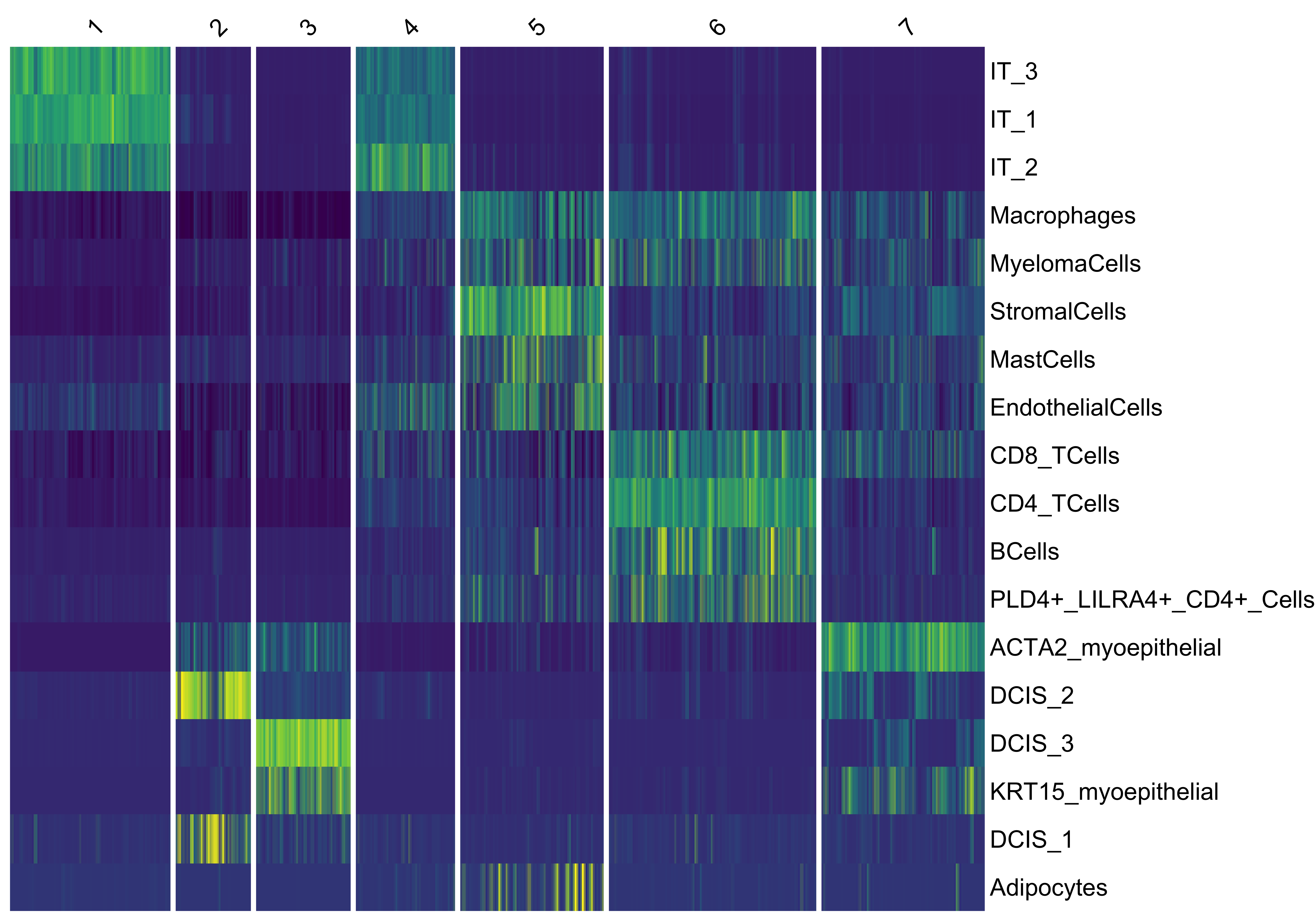
6_Assay1 6_Assay1     7   Assay1 Xenium Section1 10XBlock   DCIS_1              2

Visualization

vrSpatialPlot(Xen_data, group.by = "niche_clusters", alpha = 1, legend.loc = "top")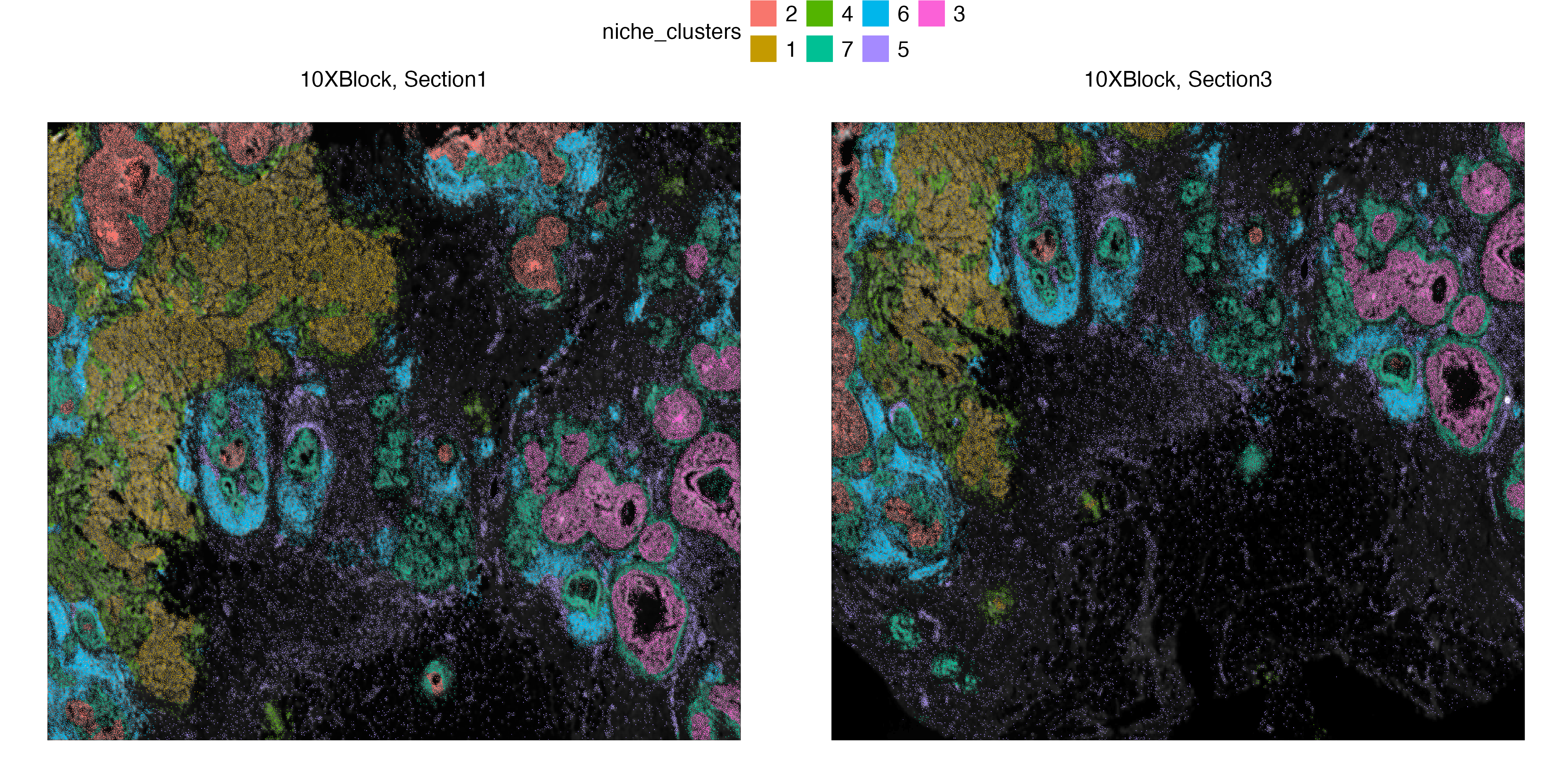

vrHeatmapPlot(Xen_data, features = vrFeatures(Xen_data), group.by = "niche_clusters")