anglemania Tutorial

Aaron Kollotzek

Max Delbrück Center for Molecular Medicine in the Helmholtz Association, Berlin, GermanyBerlin Institute for Medical Systems Biology, Berlin, Germany
aaron.kollotzek@mdc-berlin.de

Vedran Franke

Max Delbrück Center for Molecular Medicine in the Helmholtz Association, Berlin, GermanyBerlin Institute for Medical Systems Biology, Berlin, Germany

Artem Baranovskii

Helmholtz Munich

Altuna Akalin

Max Delbrück Center for Molecular Medicine in the Helmholtz Association, Berlin, GermanyBerlin Institute for Medical Systems Biology, Berlin, Germany

2025-10-23

Source: vignettes/anglemania_tutorial.Rmd

anglemania_tutorial.Rmd

Introduction

anglemania is a feature selection package that extracts genes from multi-batch scRNA-seq experiments for downstream dataset integration. The goal is to select genes that carry high biological information and low technical noise between the batches. Those genes are extracted from gene pairs that have an invariant and extremely narrow or wide angle between their expression vectors. Conventionally, highly-variable genes (HVGs) or sometimes all genes are used for integration tasks (https://www.nature.com/articles/s41592-021-01336-8). While HVGs are a great and easy way to reduce the noise and dimensionality of the data, we hypothesize that there are better ways to select genes specifically for integration tasks. HVGs are sensitive to batch effects because the variance is a function of both the technical and biological variance. anglemania improves conventional usage of HVGs for integration tasks, especially when the transcriptional difference between cell types or cell states is subtle (showcased here using simulated data generated using splatter with de.facLoc and de.facScale set to 0.1, which results in mild differences between “Groups”). The package can be used on top of SingleCellExperiment or Seurat objects.

Under the hood, anglemania works with file-backed big matrices (FBMs) from the bigstatsr package for fast and memory efficient computation.

suppressPackageStartupMessages({
    library(anglemania)
    library(dplyr)
    library(Seurat)
    options(Seurat.object.assay.version = "v5")
    library(splatter)
    library(SingleCellExperiment)
    library(scater)
    library(scran)
    library(bluster)
    library(batchelor)
    library(UpSetR)
})

Simulation

We simulate a scRNA-seq dataset using Splatter with 4 batches and 3 cell types with subtle differences between cell types and rather big batch effects.

batch.facLoc <- 0.3
de.facLoc <- 0.1
nBatches <- 4
nGroups <- 3
nGenes <- 5000
groupCells <- 300

sce_raw <- splatSimulate(
    batchCells = rep(groupCells * nGroups, nBatches),
    batch.facLoc = batch.facLoc,
    group.prob = rep(1 / nGroups, nGroups),
    nGenes = nGenes,
    batch.facScale = 0.1,
    method = "groups",
    verbose = FALSE,
    out.prob = 0.001,
    de.prob = 0.1, # mild
    de.facLoc = de.facLoc,
    de.facScale = 0.1,
    bcv.common = 0.1,
    seed = 42
)
sce <- sce_raw
assays(sce)

## List of length 6
## names(6): BatchCellMeans BaseCellMeans BCV CellMeans TrueCounts counts

Unintegrated data

Here we perform a standard workflow on the unintegrated data. When we perform clustering on the unintegrated data and visualize it in a UMAP, we can see that the clusters are driven by batch effects rather than cell types.

sce_unintegrated <- sce
# Normalization.
sce_unintegrated <- logNormCounts(sce_unintegrated)

# Feature selection.
dec <- modelGeneVar(sce_unintegrated)
hvg <- getTopHVGs(dec, prop = 0.1)

# PCA.
set.seed(1234)
sce_unintegrated <- scater::runPCA(
    sce_unintegrated,
    ncomponents = 50,
    subset_row = hvg
)

# Clustering.
colLabels(sce_unintegrated) <- clusterCells(sce_unintegrated,
    use.dimred = "PCA",
    BLUSPARAM = NNGraphParam(cluster.fun = "louvain")
)

# Visualization.
sce_unintegrated <- scater::runUMAP(sce_unintegrated, dimred = "PCA")
patchwork::wrap_plots(
    plotUMAP(sce_unintegrated, colour_by = "Batch") +
        ggtitle("Unintegrated data, colored by Batch"),
    plotUMAP(sce_unintegrated, colour_by = "Group") +
        ggtitle("Unintegrated data, colored by Group")
)

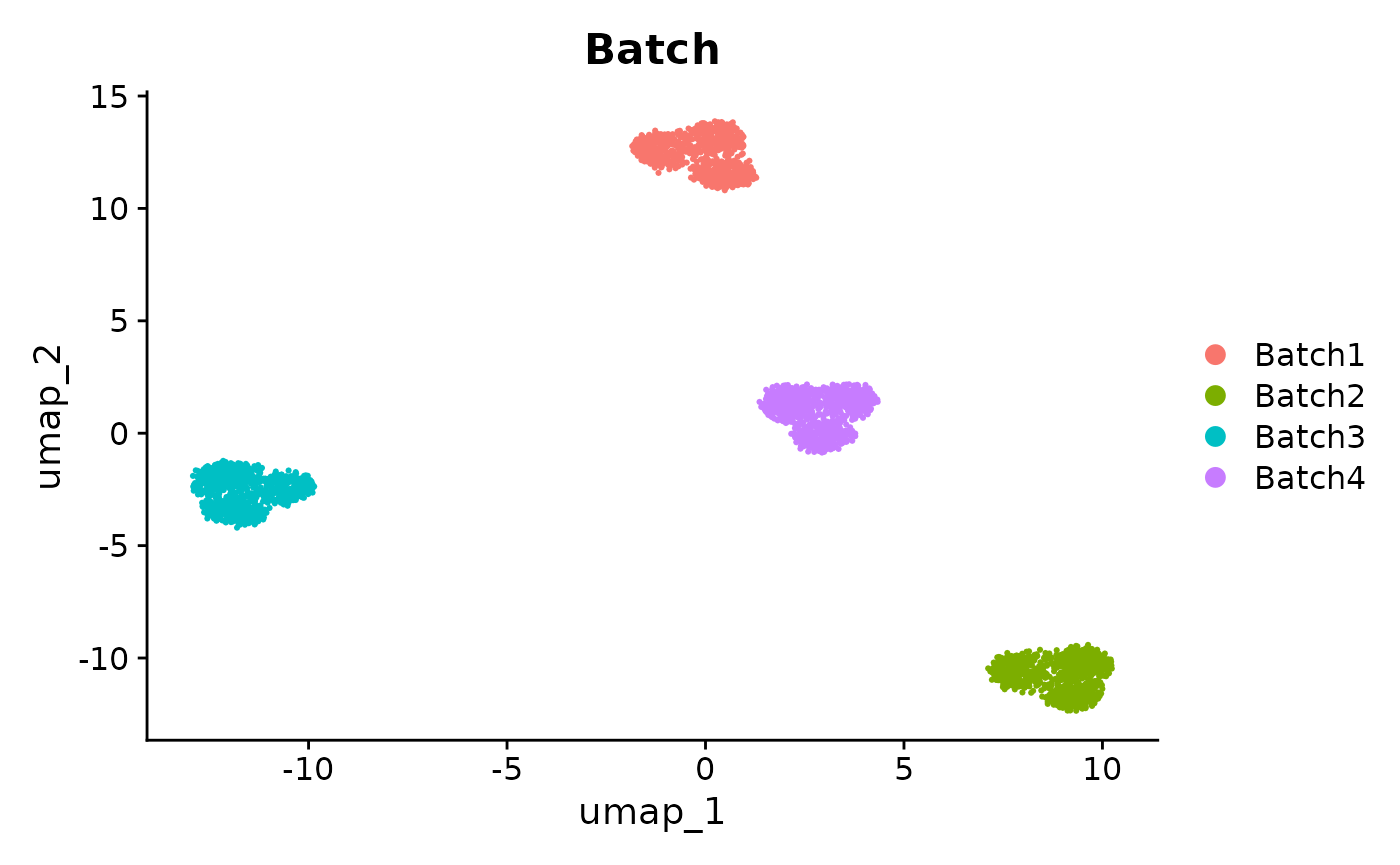
UMAPs of unintegrated data, colored by Batch and Group. The clusters are driven by batch effects.

anglemania

anglemania works on a SingleCellExperiment object. The function has a few important arguments: - batch_key: the column in the metadata of the SingleCellExperiment object that indicates which batch the cells belong to. This is required to distinguish between batches, because we compute the angle between gene pairs for each batch. - method: either cosine, spearman or diem - this is the method by which the relationship of the gene pairs is measured. Default is cosine, which is the cosine similarity between the expression vectors of the gene pairs. - max_n_genes: you can specify a maximum number of extracted genes. They are sorted by a weighted sum of the ranked mean and standard deviation of the zscores of the gene pair correlations.

head(colData(sce))

## DataFrame with 6 rows and 4 columns
##              Cell       Batch    Group ExpLibSize
##       <character> <character> <factor>  <numeric>
## Cell1       Cell1      Batch1   Group1    46898.1
## Cell2       Cell2      Batch1   Group1    54688.2
## Cell3       Cell3      Batch1   Group2    52027.9
## Cell4       Cell4      Batch1   Group1    52319.5
## Cell5       Cell5      Batch1   Group3    37774.7
## Cell6       Cell6      Batch1   Group3    58112.3

batch_key <- "Batch"
sce <- anglemania(
    sce,
    batch_key = batch_key,
    max_n_genes = 2000
)

extract the anglemania genes from the SCE object

anglemania_genes <- get_anglemania_genes(sce)
head(anglemania_genes)

## [1] "Gene527"  "Gene4620" "Gene2249" "Gene3115" "Gene2802" "Gene3566"

length(anglemania_genes)

## [1] 2000

select_genes

Once anglemania was run on the SCE, you can adjust the number of genes you want to select using the select_genes() function. It has an argument score_weights, which let’s you decide how much weight to set to the mean and standard deviation of the zscores. The default which is used in the anglemania function is 0.4 for the mean zscore and 0.6 for the standard deviation of the zscore. Higher weights for the standard deviation of the zscores lead to a greater emphasis on genes with highly stable correlation patterns.

sce <- select_genes(
    sce,
    max_n_genes = 2000,
    score_weights = c(0.4, 0.6)
)
# Inspect the anglemania genes
anglemania_genes <- get_anglemania_genes(sce)
head(anglemania_genes)

## [1] "Gene527"  "Gene4620" "Gene2249" "Gene3115" "Gene2802" "Gene3566"

length(anglemania_genes)

## [1] 2000

MNN integration

The anglemania genes can now be used for downstream integration algorithms such as MNN. We compare the integration results using the anglemania genes with the results using 500 and the standard 2000 HVGs.

HVGs

500 HVGs

hvg_500 <- sce %>%
    scater::logNormCounts() %>%
    modelGeneVar(block = colData(sce)[[batch_key]]) %>%
    getTopHVGs(n = 500)

barcodes_by_batch <- split(rownames(colData(sce)), colData(sce)[[batch_key]])
sce_list <- lapply(barcodes_by_batch, function(x) sce[, x])
sce_mnn <- sce %>%
    scater::logNormCounts()
sce_mnn <- batchelor::fastMNN(
    sce_mnn,
    subset.row = hvg_500,
    k = 20,
    batch = factor(colData(sce_mnn)[[batch_key]]),
    d = 50
)
reducedDim(sce, "MNN_hvg_500") <- reducedDim(sce_mnn, "corrected")
sce <- scater::runUMAP(sce, dimred = "MNN_hvg_500", name = "umap_MNN_hvg_500")
# k is the number of nearest neighbours to consider when identifying MNNs

2000 HVGs

hvg_2000 <- sce %>%
    scater::logNormCounts() %>%
    modelGeneVar(block = colData(sce)[[batch_key]]) %>%
    getTopHVGs(n = 2000)

barcodes_by_batch <- split(rownames(colData(sce)), colData(sce)[[batch_key]])
sce_list <- lapply(barcodes_by_batch, function(x) sce[, x])
sce_mnn <- sce %>%
    scater::logNormCounts()
sce_mnn <- batchelor::fastMNN(
    sce_mnn,
    subset.row = hvg_2000,
    k = 20,
    batch = factor(colData(sce_mnn)[[batch_key]]),
    d = 50
)
reducedDim(sce, "MNN_hvg_2000") <- reducedDim(sce_mnn, "corrected")
sce <- scater::runUMAP(sce, dimred = "MNN_hvg_2000", name = "umap_MNN_hvg_2000")

anglemania genes

sce_mnn <- sce %>%
    scater::logNormCounts()
sce_mnn <- batchelor::fastMNN(
    sce_mnn,
    subset.row = anglemania_genes,
    k = 20,
    batch = factor(colData(sce_mnn)[[batch_key]]),
    d = 50
)
reducedDim(sce, "MNN_anglemania_2000") <- reducedDim(sce_mnn, "corrected")
sce <- scater::runUMAP(
    sce,
    dimred = "MNN_anglemania_2000",
    name = "umap_MNN_anglemania_2000"
)

sce_mnn <- sce %>%
    scater::logNormCounts()
sce_mnn <- batchelor::fastMNN(
    sce_mnn,
    subset.row = anglemania_genes[1:500],
    k = 20,
    batch = factor(colData(sce_mnn)[[batch_key]]),
    d = 50
)
reducedDim(sce, "MNN_anglemania_500") <- reducedDim(sce_mnn, "corrected")
sce <- scater::runUMAP(
    sce,
    dimred = "MNN_anglemania_500",
    name = "umap_MNN_anglemania_500"
)

Plot

UMAP embeddings

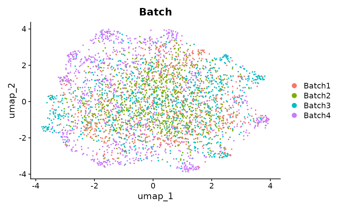
We can see from the UMAPs that anglemania genes yield the best integration in terms of clustering by cell type and mixing the batches. The goal of an integration and subsequent clustering should be to have low intra cluster variance and high inter cluster variance. This is at least true for most downstream scRNA-seq analyses where the goal is to e.g. differentiate between cell types or cell states and annotate these.

# Use wrap_plots
patchwork::wrap_plots(
    plotReducedDim(sce, colour_by = "Batch", dimred = "umap_MNN_anglemania_500") +
        ggtitle("MNN integration using 500 anglemania genes, colored by Batch"),
    plotReducedDim(sce, colour_by = "Group", dimred = "umap_MNN_anglemania_500") +
        ggtitle("MNN integration using anglemania genes, colored by Group"),
    plotReducedDim(sce, colour_by = "Batch", dimred = "umap_MNN_hvg_500") +
        ggtitle("MNN integration using top 500 HVGs, colored by Batch"),
    plotReducedDim(sce, colour_by = "Group", dimred = "umap_MNN_hvg_500") +
        ggtitle("MNN integration using top 500 HVGs, colored by Group"),
    ncol = 2
)

UMAPs of MNN integrated data. Comparison of UMAP embeddings of integrated data using anglemania genes, top 500 HVGs and top 2000 HVGs.

patchwork::wrap_plots(
    plotReducedDim(sce, colour_by = "Batch", dimred = "umap_MNN_anglemania_2000") +
        ggtitle("MNN integration using 2000 anglemania genes, colored by Batch"),
    plotReducedDim(sce, colour_by = "Group", dimred = "umap_MNN_anglemania_2000") +
        ggtitle("MNN integration using 2000 anglemania genes, colored by Group"),
    plotReducedDim(sce, colour_by = "Batch", dimred = "umap_MNN_hvg_2000") +
        ggtitle("MNN integration using top 2000 HVGs, colored by Batch"),
    plotReducedDim(sce, colour_by = "Group", dimred = "umap_MNN_hvg_2000") +
        ggtitle("MNN integration using top 2000 HVGs, colored by Group"),
    ncol = 2
)

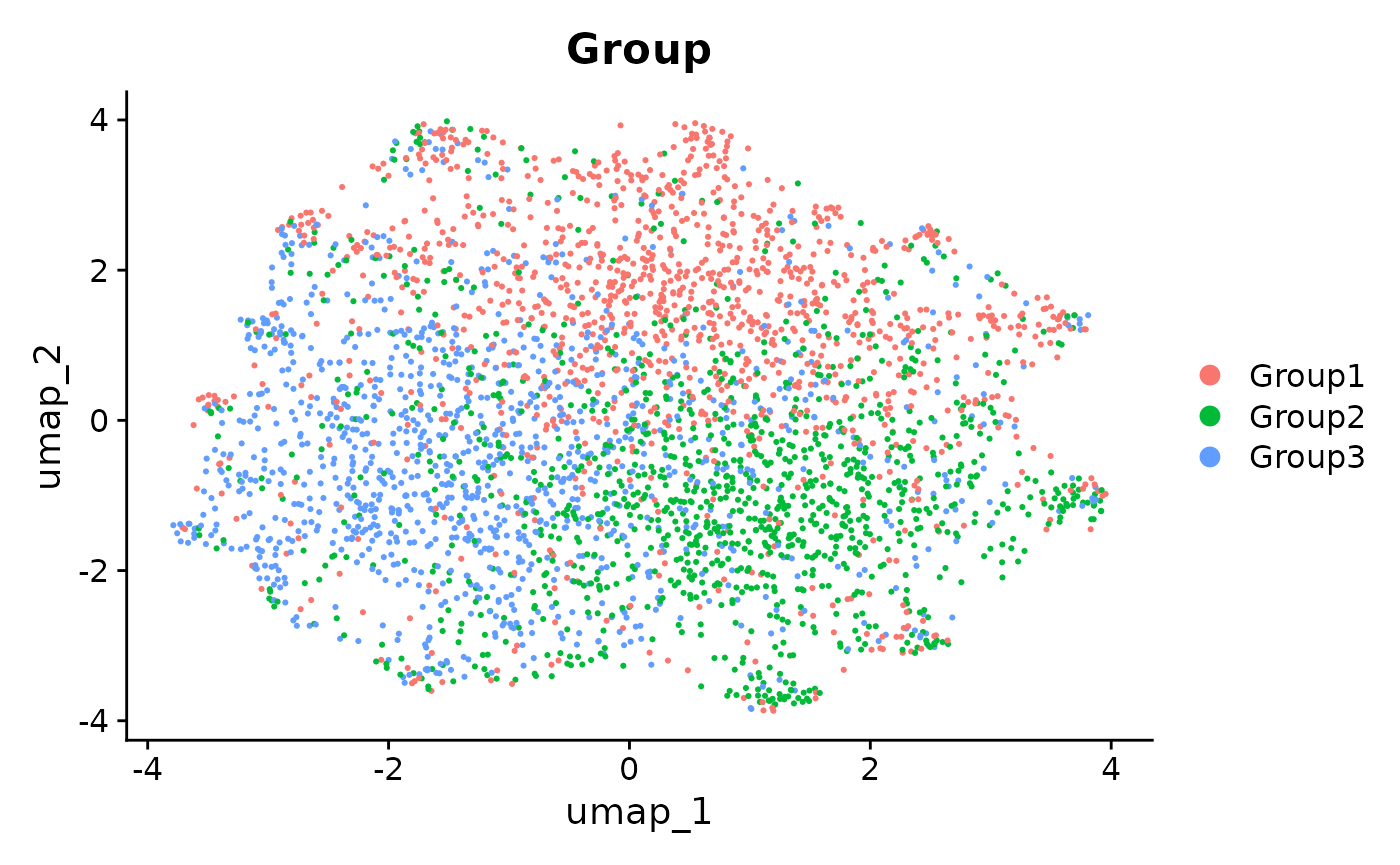
UMAPs of MNN integrated data. Comparison of UMAP embeddings of integrated data using anglemania genes, top 500 HVGs and top 2000 HVGs.

Overlap

upsetr_df <- fromList(
    list(
        anglemania = anglemania_genes,
        hvg_500 = hvg_500,
        hvg_2000 = hvg_2000
    )
)
upset(upsetr_df, text.scale = 2)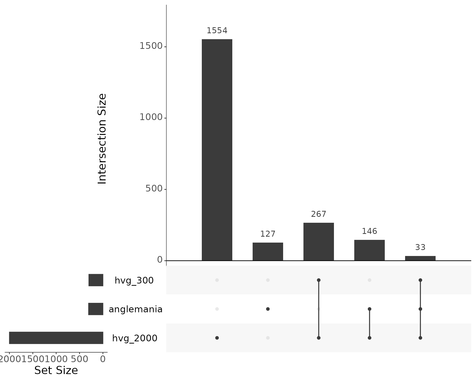

Overlap of selected genes. Additionally, we check the overlap of the anglemania genes with the HVGs. About 211 of the 2000 anglemania genes are also found in the top 500 HVGs, and 822 of the 2000 anglemania genes are also found in the top 2000 HVGs.

Seurat

Now you can just use the anglemania genes for other integration algorithms. When using Seurat, the easiest approach is to create an SCE from the counts and metadata of the SeuratObject, then run anglemania on it and save those genes as the VariableFeatures of the SeuratObject.

se <- CreateSeuratObject(
    counts = counts(sce_raw),
    meta.data = as.data.frame(colData(sce_raw))
)
se

## An object of class Seurat 
## 5000 features across 3600 samples within 1 assay 
## Active assay: RNA (5000 features, 0 variable features)
##  1 layer present: counts

anglemania_genes <- se |>
    as.SingleCellExperiment(assay = "RNA") |>
    anglemania(
        batch_key = "Batch",
        max_n_genes = 2000
    ) |>
    get_anglemania_genes()

Integration

In Seurat v5 you split the layers of an assay by batch and then run the normal Seurat workflow. To use anglemania genes for integration, you need to assign them to the VariableFeatures slot of the SeuratObject. After that, you integrate the layers using the anglemania genes as the features argument.

# Split by batch
se[["RNA"]] <- split(se[["RNA"]], f = se$Batch)

# Standard preprocessing but use anglemania genes as "VariableFeatures"
se <- NormalizeData(se, verbose = FALSE)
VariableFeatures(se) <- anglemania_genes
se <- se |>
    ScaleData(verbose = FALSE) |>
    RunPCA(verbose = FALSE)

# Integrate
se <- IntegrateLayers(
    object = se,
    method = CCAIntegration,
    orig.reduction = "pca",
    new.reduction = "integrated.cca",
    features = anglemania_genes,
    verbose = FALSE
)
se <- RunUMAP(se, dims = 1:30, reduction = "integrated.cca", verbose = FALSE)
se

## An object of class Seurat 
## 5000 features across 3600 samples within 1 assay 
## Active assay: RNA (5000 features, 2000 variable features)
##  9 layers present: counts.Batch1, counts.Batch2, counts.Batch3, counts.Batch4, data.Batch1, data.Batch2, data.Batch3, data.Batch4, scale.data
##  3 dimensional reductions calculated: pca, integrated.cca, umap

Plot

patchwork::wrap_plots(
    DimPlot(se, reduction = "umap", group.by = "Batch") +
        ggtitle("Seurat integration using\nanglemania genes\ncolored by Batch"),
    DimPlot(se, reduction = "umap", group.by = "Group") +
        ggtitle("Seurat integration using\nanglemania genes\ncolored by Group"),
    ncol = 2
)

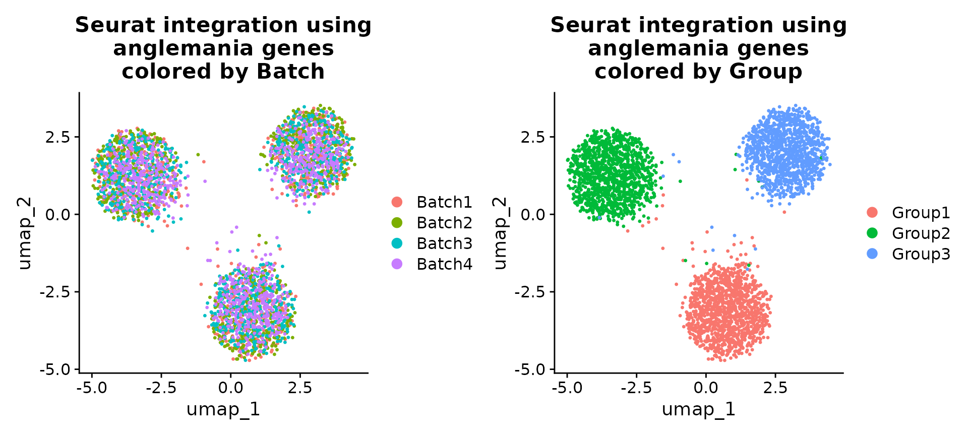
UMAPs of Seurat integrated data. Here we show that we can use the anglemania genes for integration of a SeuratObject.

Showcase underlying functions

Normal anglemania workflow

sce_raw <- sce_example()
sce <- sce_raw
batch_key <- "batch"
sce <- anglemania(sce, batch_key = batch_key, verbose = FALSE)

anglemania is run on the SCE object and it basically calls three functions:

factorise:
- creates a permutation of the input matrix whose correlation matrix is used to create a null distribution for each batch.
- computes the cosine similarity (or spearman coefficient) between gene expression vector pairs matrix for both the original and permuted matrices
- computes the zscore of the relationship between the gene pairs taking the mean and standard deviation of the null distribution
- it does this for every batch in the dataset!
get_list_stats
- computes the mean and standard deviation of the zscores across the matrices from the different batches. This creates two important matrices: the mean zscore matrix mean_zscore and the signal-to-noise ratio matrix sn_zscore. These are stored in the metadata of the SCE object.
select_genes
- filters the gene pairs by the mean_zscore and sn_zscore matrices (SN ratio, i.e. the mean divided by the standard deviation).

factorise

barcodes_by_batch <- split(rownames(colData(sce)), colData(sce)[[batch_key]])
counts_by_batch <- lapply(barcodes_by_batch, function(x) {
    counts(sce[, x]) %>% sparse_to_fbm()
})
counts_by_batch[[1]][1:10, 1:6]

##       [,1] [,2] [,3] [,4] [,5] [,6]
##  [1,]    8    5    5    2    4    2
##  [2,]    9    5    4    1    4    9
##  [3,]    4    2    7    4    6    1
##  [4,]    7    4    4    1    3    8
##  [5,]    6    8    5    5    7    4
##  [6,]    5    8    5    9    8    6
##  [7,]    6    4    7    4    7    5
##  [8,]    3    3    3    3    5    4
##  [9,]    6    4    5    5    3    1
## [10,]    6    4    5    2    6    4

# we are working on FBMs (file-backed matrices
# implemented in the bigstatsr package)
class(counts_by_batch[[1]])

## [1] "FBM"
## attr(,"package")
## [1] "bigstatsr"

# factorise produces the correlation matrices transformed to z-scores
factorised <- lapply(counts_by_batch, factorise)
factorised[[1]][1:10, 1:6]

##              [,1]        [,2]        [,3]       [,4]       [,5]        [,6]
##  [1,]  0.00000000 -1.74668209 -0.79613304  1.1776966  0.8601212  0.50193905
##  [2,] -1.73785984  0.00000000  0.59661885  2.5115045  0.5348975  1.43483620
##  [3,] -0.85963025  0.53988067  0.00000000  0.2901283 -1.5767324 -0.06260101
##  [4,]  1.13658651  2.45514150  0.33158301  0.0000000 -0.3715653 -0.57325460
##  [5,]  0.92122274  0.57796947 -1.62420449 -0.3961608  0.0000000 -0.26750572
##  [6,]  0.52925575  1.57028828 -0.02415793 -0.6582967 -0.2979901  0.00000000
##  [7,] -0.41325531 -0.10548957 -1.16180200  0.0055108  0.3444741  1.41598180
##  [8,]  0.10001406 -1.38192310 -1.29577006 -0.2524730 -0.7968541 -1.56575595
##  [9,]  0.51996703  0.05963883 -0.37002326 -0.2927571 -0.9185203 -0.12159157
## [10,]  0.06970488 -0.33637803  1.57056534  0.3728527  0.5142178  1.01784989

get_list_stats

The “list stats” are computed by get_list_stats and take the z-score transformed correlation matrices from factorise as input. The outputs are the mean zscore matrix mean_zscore and the signal-to-noise ratio matrix sn_zscore. These are stored in the metadata of the SCE object.

matrix_list <- metadata(sce)$anglemania$matrix_list
weights <- setNames(
    metadata(sce)$anglemania$params$dataset_weights$weight,
    metadata(sce)$anglemania$params$dataset_weights$anglemania_batch
)
list_stats <- get_list_stats(
    matrix_list = matrix_list,
    weights = weights,
    verbose = FALSE
)
names(list_stats)

## [1] "mean_zscore" "sds_zscore"  "sn_zscore"

class(list_stats)

## [1] "list"

list_stats$mean_zscore[1:10, 1:6]

##              [,1]       [,2]       [,3]        [,4]        [,5]       [,6]
##  [1,]  0.00000000 -1.4773877 -0.6690115  0.80957395  0.21191114  0.3065459
##  [2,] -1.43297508  0.0000000  0.8094372  1.79591873  0.87491750  0.0903189
##  [3,] -0.70975605  0.8090174  0.0000000 -0.90002758 -0.14215190  0.4217798
##  [4,]  0.81025807  1.7916458 -0.8103351  0.00000000 -0.29386285 -0.2877692
##  [5,]  0.26228504  0.8796571 -0.2190412 -0.31429554  0.00000000 -0.7944232
##  [6,]  0.34210706  0.1727196  0.4235970 -0.32724467 -0.79625202  0.0000000
##  [7,]  0.60813294  0.4576137 -1.4403958 -0.03807431  0.35694728  0.5394522
##  [8,] -0.03868058 -1.0958225 -0.7680151 -0.62207485 -1.42724690 -0.8197054
##  [9,]  1.26715940  0.3486664 -0.5030029 -0.76152650 -0.66668260 -0.4825756
## [10,]  0.49115807  1.1467226  0.7976727 -0.27013900  0.03028304  0.8112288

list_stats$sn_zscore[1:10, 1:6]

##            [,1]       [,2]      [,3]      [,4]        [,5]      [,6]
##  [1,]        NA 3.87928890 3.7213414 1.5550667  0.23116551 1.1093569
##  [2,] 3.3234406         NA 2.6894229 1.7746389  1.81948152 0.0475004
##  [3,] 3.3486305 2.12554305        NA 0.5347330  0.07006687 0.6157208
##  [4,] 1.7557127 1.90940919 0.5017815        NA  2.67420836 0.7127632
##  [5,] 0.2814584 2.06177351 0.1102260 2.7147101          NA 1.0660911
##  [6,] 1.2925884 0.08738832 0.6689559 0.6989744  1.12999842        NA
##  [7,] 0.4210103 0.57464016 3.6559091 0.6177018 20.23533063 0.4351825
##  [8,] 0.1972052 2.70836022 1.0290168 1.1901274  1.60093202 0.7769169
##  [9,] 1.1991785 0.85301337 2.6746701 1.1487110  1.87190277 0.9452842
## [10,] 0.8240564 0.54672981 0.7297777 0.2970755  0.04424840 2.7762187

# Or we can access them directly from the SCE object
# after running anglemania
metadata(sce)$anglemania$list_stats$mean_zscore[1:10, 1:6]

##              [,1]       [,2]       [,3]        [,4]        [,5]       [,6]
##  [1,]  0.00000000 -1.4773877 -0.6690115  0.80957395  0.21191114  0.3065459
##  [2,] -1.43297508  0.0000000  0.8094372  1.79591873  0.87491750  0.0903189
##  [3,] -0.70975605  0.8090174  0.0000000 -0.90002758 -0.14215190  0.4217798
##  [4,]  0.81025807  1.7916458 -0.8103351  0.00000000 -0.29386285 -0.2877692
##  [5,]  0.26228504  0.8796571 -0.2190412 -0.31429554  0.00000000 -0.7944232
##  [6,]  0.34210706  0.1727196  0.4235970 -0.32724467 -0.79625202  0.0000000
##  [7,]  0.60813294  0.4576137 -1.4403958 -0.03807431  0.35694728  0.5394522
##  [8,] -0.03868058 -1.0958225 -0.7680151 -0.62207485 -1.42724690 -0.8197054
##  [9,]  1.26715940  0.3486664 -0.5030029 -0.76152650 -0.66668260 -0.4825756
## [10,]  0.49115807  1.1467226  0.7976727 -0.27013900  0.03028304  0.8112288

metadata(sce)$anglemania$list_stats$sn_zscore[1:10, 1:6]

##            [,1]       [,2]      [,3]      [,4]        [,5]      [,6]
##  [1,]        NA 3.87928890 3.7213414 1.5550667  0.23116551 1.1093569
##  [2,] 3.3234406         NA 2.6894229 1.7746389  1.81948152 0.0475004
##  [3,] 3.3486305 2.12554305        NA 0.5347330  0.07006687 0.6157208
##  [4,] 1.7557127 1.90940919 0.5017815        NA  2.67420836 0.7127632
##  [5,] 0.2814584 2.06177351 0.1102260 2.7147101          NA 1.0660911
##  [6,] 1.2925884 0.08738832 0.6689559 0.6989744  1.12999842        NA
##  [7,] 0.4210103 0.57464016 3.6559091 0.6177018 20.23533063 0.4351825
##  [8,] 0.1972052 2.70836022 1.0290168 1.1901274  1.60093202 0.7769169
##  [9,] 1.1991785 0.85301337 2.6746701 1.1487110  1.87190277 0.9452842
## [10,] 0.8240564 0.54672981 0.7297777 0.2970755  0.04424840 2.7762187

select_genes

under the hood, anglemania calls select_genes
we can use select_genes to change the number of selected genes without having to run anglemania again

previous_genes <- get_anglemania_genes(sce)
sce <- select_genes(
    sce,
    max_n_genes = 2000,
    verbose = FALSE
)
# Inspect the anglemania genes
new_genes <- get_anglemania_genes(sce)

length(previous_genes)

## [1] 300

length(new_genes)

## [1] 300

sessionInfo

sessionInfo()

## R version 4.5.1 (2025-06-13)
## Platform: x86_64-pc-linux-gnu
## Running under: Ubuntu 24.04.3 LTS
## 
## Matrix products: default
## BLAS:   /usr/lib/x86_64-linux-gnu/openblas-pthread/libblas.so.3 
## LAPACK: /usr/lib/x86_64-linux-gnu/openblas-pthread/libopenblasp-r0.3.26.so;  LAPACK version 3.12.0
## 
## locale:
##  [1] LC_CTYPE=C.UTF-8       LC_NUMERIC=C           LC_TIME=C.UTF-8       
##  [4] LC_COLLATE=C.UTF-8     LC_MONETARY=C.UTF-8    LC_MESSAGES=C.UTF-8   
##  [7] LC_PAPER=C.UTF-8       LC_NAME=C              LC_ADDRESS=C          
## [10] LC_TELEPHONE=C         LC_MEASUREMENT=C.UTF-8 LC_IDENTIFICATION=C   
## 
## time zone: UTC
## tzcode source: system (glibc)
## 
## attached base packages:
## [1] stats4    stats     graphics  grDevices utils     datasets  methods  
## [8] base     
## 
## other attached packages:
##  [1] future_1.67.0               UpSetR_1.4.0               
##  [3] batchelor_1.24.0            bluster_1.18.0             
##  [5] scran_1.36.0                scater_1.36.0              
##  [7] ggplot2_4.0.0               scuttle_1.18.0             
##  [9] splatter_1.32.0             SingleCellExperiment_1.30.1
## [11] SummarizedExperiment_1.38.1 Biobase_2.68.0             
## [13] GenomicRanges_1.60.0        GenomeInfoDb_1.44.3        
## [15] IRanges_2.42.0              S4Vectors_0.46.0           
## [17] BiocGenerics_0.54.1         generics_0.1.4             
## [19] MatrixGenerics_1.20.0       matrixStats_1.5.0          
## [21] Seurat_5.3.0                SeuratObject_5.2.0         
## [23] sp_2.2-0                    dplyr_1.1.4                
## [25] anglemania_0.99.7           BiocStyle_2.36.0           
## 
## loaded via a namespace (and not attached):
##   [1] RcppAnnoy_0.0.22          splines_4.5.1            
##   [3] later_1.4.4               tibble_3.3.0             
##   [5] polyclip_1.10-7           fastDummies_1.7.5        
##   [7] lifecycle_1.0.4           edgeR_4.6.3              
##   [9] doParallel_1.0.17         globals_0.18.0           
##  [11] lattice_0.22-7            MASS_7.3-65              
##  [13] backports_1.5.0           magrittr_2.0.4           
##  [15] limma_3.64.3              plotly_4.11.0            
##  [17] sass_0.4.10               rmarkdown_2.30           
##  [19] jquerylib_0.1.4           yaml_2.3.10              
##  [21] bigparallelr_0.3.2        metapod_1.16.0           
##  [23] httpuv_1.6.16             otel_0.2.0               
##  [25] sctransform_0.4.2         spam_2.11-1              
##  [27] spatstat.sparse_3.1-0     reticulate_1.43.0        
##  [29] cowplot_1.2.0             pbapply_1.7-4            
##  [31] RColorBrewer_1.1-3        ResidualMatrix_1.18.0    
##  [33] abind_1.4-8               Rtsne_0.17               
##  [35] purrr_1.1.0               bigassertr_0.1.7         
##  [37] GenomeInfoDbData_1.2.14   ggrepel_0.9.6            
##  [39] irlba_2.3.5.1             listenv_0.9.1            
##  [41] spatstat.utils_3.2-0      goftest_1.2-3            
##  [43] RSpectra_0.16-2           dqrng_0.4.1              
##  [45] spatstat.random_3.4-2     fitdistrplus_1.2-4       
##  [47] parallelly_1.45.1         DelayedMatrixStats_1.30.0
##  [49] pkgdown_2.1.3             codetools_0.2-20         
##  [51] DelayedArray_0.34.1       tidyselect_1.2.1         
##  [53] UCSC.utils_1.4.0          farver_2.1.2             
##  [55] viridis_0.6.5             ScaledMatrix_1.16.0      
##  [57] bigstatsr_1.6.2           spatstat.explore_3.5-3   
##  [59] flock_0.7                 jsonlite_2.0.0           
##  [61] BiocNeighbors_2.2.0       progressr_0.17.0         
##  [63] ggridges_0.5.7            survival_3.8-3           
##  [65] iterators_1.0.14          systemfonts_1.3.1        
##  [67] foreach_1.5.2             tools_4.5.1              
##  [69] ragg_1.5.0                ica_1.0-3                
##  [71] Rcpp_1.1.0                glue_1.8.0               
##  [73] gridExtra_2.3             SparseArray_1.8.1        
##  [75] xfun_0.53                 withr_3.0.2              
##  [77] BiocManager_1.30.26       fastmap_1.2.0            
##  [79] rsvd_1.0.5                digest_0.6.37            
##  [81] R6_2.6.1                  mime_0.13                
##  [83] textshaping_1.0.4         scattermore_1.2          
##  [85] tensor_1.5.1              spatstat.data_3.1-9      
##  [87] tidyr_1.3.1               data.table_1.17.8        
##  [89] FNN_1.1.4.1               httr_1.4.7               
##  [91] htmlwidgets_1.6.4         S4Arrays_1.8.1           
##  [93] uwot_0.2.3                pkgconfig_2.0.3          
##  [95] gtable_0.3.6              lmtest_0.9-40            
##  [97] S7_0.2.0                  XVector_0.48.0           
##  [99] htmltools_0.5.8.1         dotCall64_1.2            
## [101] bookdown_0.45             scales_1.4.0             
## [103] png_0.1-8                 spatstat.univar_3.1-4    
## [105] knitr_1.50                reshape2_1.4.4           
## [107] checkmate_2.3.3           nlme_3.1-168             
## [109] cachem_1.1.0              zoo_1.8-14               
## [111] stringr_1.5.2             rmio_0.4.0               
## [113] KernSmooth_2.23-26        vipor_0.4.7              
## [115] parallel_4.5.1            miniUI_0.1.2             
## [117] desc_1.4.3                pillar_1.11.1            
## [119] grid_4.5.1                vctrs_0.6.5              
## [121] RANN_2.6.2                promises_1.4.0           
## [123] BiocSingular_1.24.0       ff_4.5.2                 
## [125] beachmat_2.24.0           xtable_1.8-4             
## [127] cluster_2.1.8.1           beeswarm_0.4.0           
## [129] evaluate_1.0.5            cli_3.6.5                
## [131] locfit_1.5-9.12           compiler_4.5.1           
## [133] rlang_1.1.6               crayon_1.5.3             
## [135] future.apply_1.20.0       labeling_0.4.3           
## [137] ps_1.9.1                  ggbeeswarm_0.7.2         
## [139] plyr_1.8.9                fs_1.6.6                 
## [141] stringi_1.8.7             viridisLite_0.4.2        
## [143] deldir_2.0-4              BiocParallel_1.42.2      
## [145] lazyeval_0.2.2            spatstat.geom_3.6-0      
## [147] Matrix_1.7-3              RcppHNSW_0.6.0           
## [149] patchwork_1.3.2           sparseMatrixStats_1.20.0 
## [151] statmod_1.5.1             shiny_1.11.1             
## [153] ROCR_1.0-11               igraph_2.2.0             
## [155] bslib_0.9.0               bit_4.6.0