cacheR automatically tracks which cached function called which and which files each depends on. This vignette explores the full graph API: building, inspecting, persisting, and visualising the dependency DAG.
1. Building a Pipeline
When a cached function calls another cached function, cacheR records the parent → child relationship automatically.
library(cacheR)

cache_dir <- file.path(tempdir(), "graph_demo")
if (dir.exists(cache_dir)) unlink(cache_dir, recursive = TRUE)
cacheTree_reset()

load_counts <- cacheFile(cache_dir, backend = "rds") %@% function(path) {
  list(genes = c("TP53", "BRCA1", "EGFR"), counts = c(100, 250, 80))
}

normalize <- cacheFile(cache_dir, backend = "rds") %@% function(counts) {
  total <- sum(counts$counts)
  setNames(counts$counts / total, counts$genes)
}

top_genes <- cacheFile(cache_dir, backend = "rds") %@% function(normed, n = 2) {
  head(sort(normed, decreasing = TRUE), n)
}

pipeline <- cacheFile(cache_dir, backend = "rds") %@% function(input_path, n = 2) {
  raw <- load_counts(input_path)
  normed <- normalize(raw)
  top_genes(normed, n = n)
}

result <- pipeline("samples/counts.csv")
print(result)
#>     BRCA1      TP53
#> 0.5813953 0.2325581
2. Inspecting Nodes
Each node stores: function name, hash, parent/child links, tracked files, and cache file path.
nodes <- cacheTree_nodes()
cat(sprintf("Total nodes: %d\n\n", length(nodes)))
#> Total nodes: 4

for (nid in names(nodes)) {
  nd <- nodes[[nid]]
  cat(sprintf("Node: %s\n", nd$fname))
  cat(sprintf("  ID:       %s\n", nid))
  cat(sprintf("  Parents:  %s\n", paste(nd$parents, collapse = ", ")))
  cat(sprintf("  Children: %s\n", paste(nd$children, collapse = ", ")))
  cat(sprintf("  Files:    %s\n", paste(nd$files, collapse = ", ")))
  cat("\n")
}
#>   ID:       top_genes_af4a5e7f03ea1d03
#>   Parents:  pipeline_2fe7d5d69daeb6f1
#>   Children:
#>   Files:
#>
#>   ID:       pipeline_2fe7d5d69daeb6f1
#>   Parents:
#>   Children: load_counts_b12c6ab05e654db1, normalize_851b9dd2ac5ddd84, top_genes_af4a5e7f03ea1d03
#>   Files:
#>
#>   ID:       normalize_851b9dd2ac5ddd84
#>   Parents:  pipeline_2fe7d5d69daeb6f1
#>   Children:
#>   Files:
#>
#>   ID:       load_counts_b12c6ab05e654db1
#>   Parents:  pipeline_2fe7d5d69daeb6f1
#>   Children:
#>   Files:
3. File Tracking with track_file()
track_file(path) registers an explicit file dependency
on the current graph node.
cacheTree_reset()
cache_dir2 <- file.path(tempdir(), "graph_demo_files")
if (dir.exists(cache_dir2)) unlink(cache_dir2, recursive = TRUE)

data_file <- file.path(tempdir(), "demo_data.tsv")
writeLines("gene\tcount\nTP53\t100\nBRCA1\t250", data_file)

read_data <- cacheFile(cache_dir2, backend = "rds") %@% function(path) {
  track_file(path)
  read.delim(path, sep = "\t")
}

summarize_data <- cacheFile(cache_dir2, backend = "rds") %@% function(path) {
  df <- read_data(path)
  setNames(df$count, df$gene)
}

print(summarize_data(data_file))
#>  TP53 BRCA1
#>   100   250

# Show tracked files
nodes <- cacheTree_nodes()
for (nid in names(nodes)) {
  nd <- nodes[[nid]]
  fh <- nd$file_hashes
  if (length(fh) > 0) {
    cat(sprintf("\n%s tracks %d file(s):\n", nd$fname, length(fh)))
    for (fp in names(fh)) {
      cat(sprintf("  %s  hash=%s...\n", fp, substr(fh[[fp]], 1, 16)))
    }
  }
}
#>   /tmp/RtmpM3FfoQ/demo_data.tsv  hash=f2e3d9f280db769d...
#>   /tmp/RtmpM3FfoQ/demo_data.tsv  hash=f2e3d9f280db769d...
4. Staleness Detection
cache_tree_changed_files() compares stored hashes
against current disk state.
# Before modification
stale <- cache_tree_changed_files()
cat(sprintf("Stale nodes before edit: %d\n", length(stale)))
#> Stale nodes before edit: 0
# Modify the file
writeLines("gene\tcount\nTP53\t100\nBRCA1\t250\nEGFR\t500", data_file)
stale <- cache_tree_changed_files()
cat(sprintf("Stale nodes after edit: %d\n", length(stale)))
#> Stale nodes after edit: 2
for (nid in names(stale)) {
cat(sprintf(" %s: %s\n", stale[[nid]]$node$fname,
paste(stale[[nid]]$changed_files, collapse = ", ")))
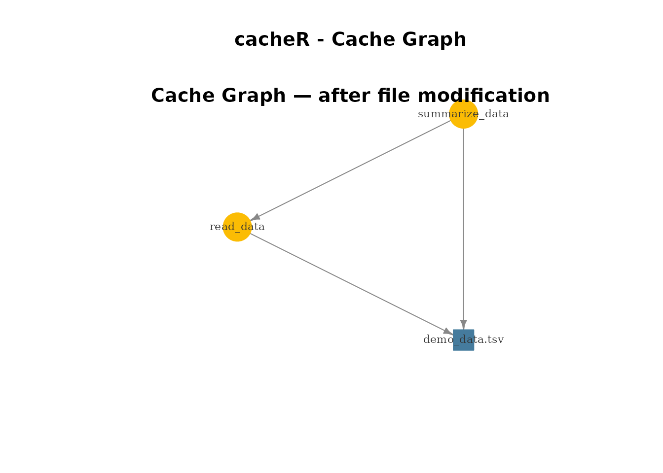
}5. Visualisation
plot_cache_graph() renders the DAG with igraph.
- Navy = cached and up-to-date
- Amber = stale (tracked file changed)
- Blue = tracked file node
- Gray = cache file missing
if (requireNamespace("igraph", quietly = TRUE)) {
  plot_cache_graph()
  mtext("Cache Graph — after file modification", side = 3, line = -1.5, cex = 1.2, font = 2)
}
Save to file:
plot_cache_graph(output = "my_graph.png")6. Graph Persistence
The graph can be saved and loaded independently of the cache files.
save_path <- file.path(tempdir(), "my_graph.rds")

# Save
cacheTree_save(save_path)
cat(sprintf("Saved %d nodes to %s\n", length(cacheTree_nodes()), save_path))
#> Saved 3 nodes to /tmp/RtmpM3FfoQ/my_graph.rds

# Reset and verify
cacheTree_reset()
cat(sprintf("After reset: %d nodes\n", length(cacheTree_nodes())))
#> After reset: 0 nodes

# Load back
cacheTree_load(save_path)
cat(sprintf("After load:  %d nodes\n", length(cacheTree_nodes())))
#> After load:  3 nodes

# Sync merges disk graph into memory (non-destructive)
cacheTree_reset()
cacheTree_sync(cache_dir2)
cat(sprintf("After sync:  %d nodes\n", length(cacheTree_nodes())))
#> After sync:  3 nodes
7. Querying by File
cacheTree_for_file(path) finds all nodes that depend on
a specific file.
dependents <- cacheTree_for_file(normalizePath(data_file))
cat(sprintf("Nodes depending on %s:\n", basename(data_file)))
#> Nodes depending on demo_data.tsv:
for (nid in names(dependents)) {
cat(sprintf(" %s\n", dependents[[nid]]$fname))
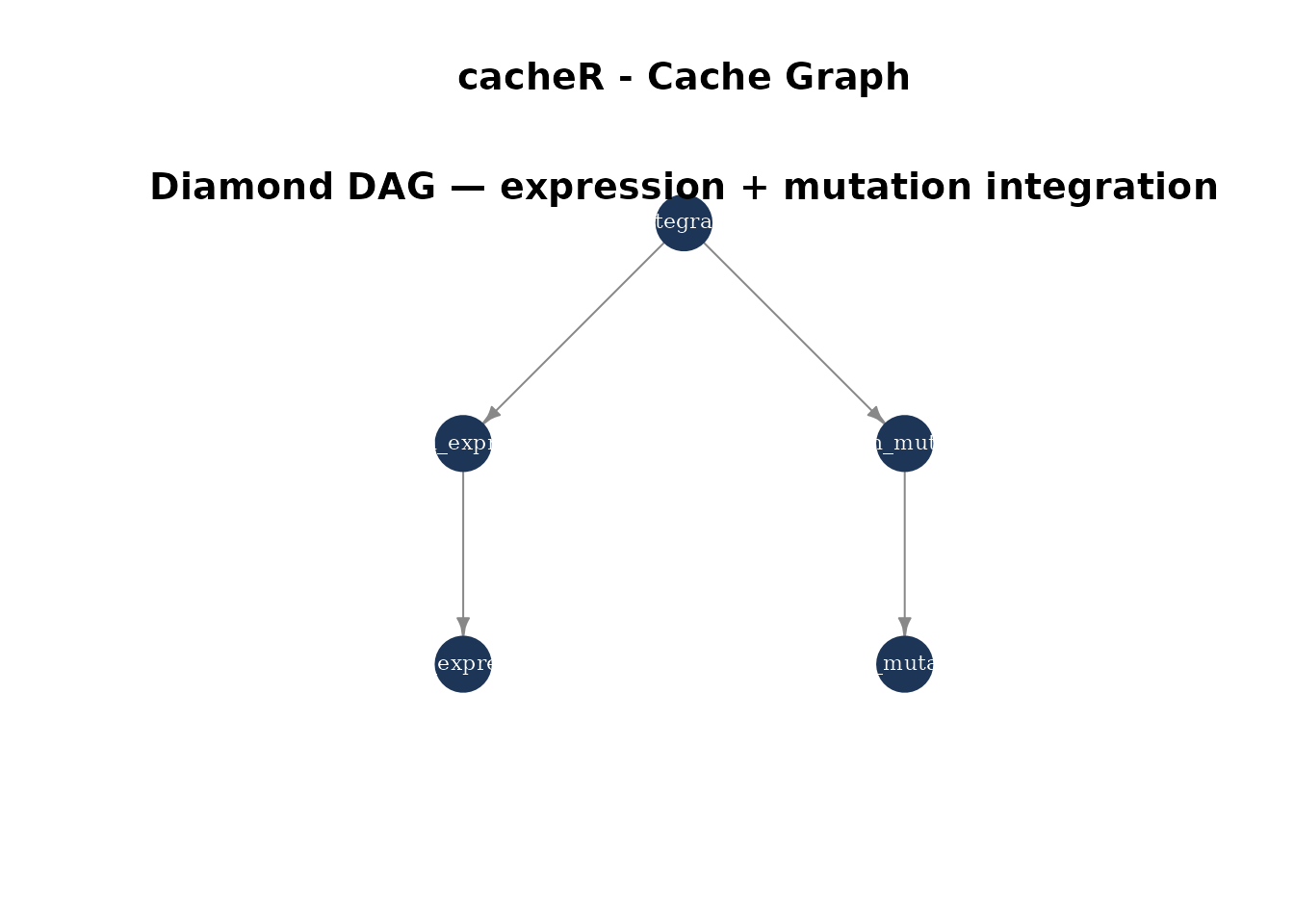
}8. Complex DAG
Build a diamond dependency: two branches merge into a final step.
cacheTree_reset()
cache_dir3 <- file.path(tempdir(), "graph_demo_diamond")
if (dir.exists(cache_dir3)) unlink(cache_dir3, recursive = TRUE)

fetch_expression <- cacheFile(cache_dir3, backend = "rds") %@% function(sample) {
  c(TP53 = 10, BRCA1 = 25, EGFR = 8)
}

fetch_mutations <- cacheFile(cache_dir3, backend = "rds") %@% function(sample) {
  c(TP53 = TRUE, BRCA1 = FALSE, EGFR = TRUE)
}

branch_expression <- cacheFile(cache_dir3, backend = "rds") %@% function(sample) {
  expr <- fetch_expression(sample)
  expr[expr > 9]
}

branch_mutations <- cacheFile(cache_dir3, backend = "rds") %@% function(sample) {
  muts <- fetch_mutations(sample)
  names(muts[muts == TRUE])
}

integrate <- cacheFile(cache_dir3, backend = "rds") %@% function(sample) {
  high_expr <- branch_expression(sample)
  mutated <- branch_mutations(sample)
  high_expr[names(high_expr) %in% mutated]
}

result <- integrate("patient_001")
cat("Genes with high expression AND mutations:\n")
#> Genes with high expression AND mutations:
print(result)
#> TP53
#>   10
cat(sprintf("\nNodes: %d\n", length(cacheTree_nodes())))
#>
#> Nodes: 5
for (nid in names(cacheTree_nodes())) {
  nd <- cacheTree_nodes()[[nid]]
  cat(sprintf("  %-25s  children=%d  parents=%d\n",
      nd$fname, length(nd$children), length(nd$parents)))
}
if (requireNamespace("igraph", quietly = TRUE)) {
  plot_cache_graph()
  mtext("Diamond DAG — expression + mutation integration", side = 3, line = -1.5, cex = 1.2, font = 2)
}
9. Graph Utilities
List all tracked files
cache_tree_files() returns a sorted vector of every file
tracked across all nodes:
Print a summary
cache_tree_summary() gives a quick overview of the full
graph:
cache_tree_summary()
#> Cache tree: 5 node(s)
#>
#>   ?
#>     id:       branch_mutations_759123e98d3ee5de
#>     parents:  integrate_baa1f2474fec17e0
#>     children: fetch_mutations_d1651aa9075de899
#>
#>   ?
#>     id:       fetch_expression_4a4b23b3d1602720
#>     parents:  branch_expression_34dc19c6325a1267
#>
#>   ?
#>     id:       fetch_mutations_d1651aa9075de899
#>     parents:  branch_mutations_759123e98d3ee5de
#>
#>   ?
#>     id:       branch_expression_34dc19c6325a1267
#>     parents:  integrate_baa1f2474fec17e0
#>     children: fetch_expression_4a4b23b3d1602720
#>
#>   ?
#>     id:       integrate_baa1f2474fec17e0
#>     children: branch_expression_34dc19c6325a1267, branch_mutations_759123e98d3ee5de
#>
10. Graph Export
JSON
cache_tree_to_json() exports nodes and edges as portable
JSON — easy to load in Python, JavaScript, or any downstream tool:
json_path <- file.path(tempdir(), "graph.json")
cache_tree_to_json(json_path)
cat(readLines(json_path, n = 20), sep = "\n")
#> {
#>   "nodes": [
#>     {
#>       "id": "branch_mutations_759123e98d3ee5de",
#>       "fname": {},
#>       "outfile": {},
#>       "parents": [
#>         "integrate_baa1f2474fec17e0"
#>       ],
#>       "children": [
#>         "fetch_mutations_d1651aa9075de899"
#>       ],
#>       "files": [],
#>       "file_hashes": []
#>     },
#>     {
#>       "id": "fetch_expression_4a4b23b3d1602720",
#>       "fname": {},
#>       "outfile": {},
#>       "parents": [
cat("...\n")
#> ...
Graphviz DOT
cache_tree_to_dot() exports the graph in DOT format for
rendering with dot, neato, or any
Graphviz-compatible tool:
dot_path <- file.path(tempdir(), "graph.dot")
cache_tree_to_dot(dot_path)
cat(readLines(dot_path), sep = "\n")
#> digraph cache_tree {
#>   rankdir=TB;
#>   node [shape=box, style=filled, fillcolor="#1D3557", fontcolor=white, fontname="sans-serif"];
#>   "integrate_baa1f2474fec17e0" -> "branch_expression_34dc19c6325a1267";
#>   "branch_mutations_759123e98d3ee5de" -> "fetch_mutations_d1651aa9075de899";
#>   "integrate_baa1f2474fec17e0" -> "branch_mutations_759123e98d3ee5de";
#>   "branch_expression_34dc19c6325a1267" -> "fetch_expression_4a4b23b3d1602720";
#> }
You can render this with Graphviz:
targets
export_targets_file() converts the cacheR graph into a
targets pipeline
script. This is useful when you want to move from interactive
exploration to a production pipeline:
targets_path <- file.path(tempdir(), "_targets.R")
export_targets_file(targets_path)
#> Exported 5 targets to /tmp/RtmpM3FfoQ/_targets.R
cat(readLines(targets_path), sep = "\n")
#> library(targets)
#> library(tarchetypes)
#> tar_option_set(packages = c('base'))
#>
#> list(
#>   tar_target(name = branch_expression, command = { branch_expression(sample) }),
#>
#>   tar_target(name = branch_mutations, command = { branch_mutations(sample) }),
#>
#>   tar_target(name = fetch_expression, command = { fetch_expression(sample) }),
#>
#>   tar_target(name = fetch_mutations, command = { fetch_mutations(sample) }),
#>
#>   tar_target(name = integrate, command = { integrate("patient_001") })
#> )
The generated _targets.R can be used directly with
targets::tar_make().